Hey Fathomlanders, how’s it going?  CoVid got you down? Need some pick-me up?  Well Fathom has just what the doctor ordered!  A full dose of  tech-talk and quasi-science-fiction.

Quasi-Science-Fiction and Cultural Artefacts

This just in! For those of you clambering for the separation of Art & Science, we now have a solution: more of both! The Sounding Posting will now be Company and Technology Reporting; the new Resonance Posting will contain Flights of Fancy, Ramblings, Shouts & Murmurs, Clubs such as Alpha (Fe)male Science Fiction Movie Club, Book Club, and Game Club.  Watch for top ten lists and vote on your favourite.  Each month, we’ll attempt to co-watch something either through Teleparty, or on your own.  We’ll open the comment lines to get some CoVid Friendly discussion going online.  Feel free to suggest other co-operatives things to do like gaming.

And most importantly, the new Fathom Cultural Artefacts Shop.  Many of you have commented on how cool my hoodie was, well now YOU can be cool too!  For just $42[efn_note]Everything is $42, even the cheap stuff, that’s called a business model[/efn_note]  you can seem like you are part of the Kool Kid’s Klub.  Christmas is coming and wouldn’t your fam and chums think you were super fresh if you gave them a Fathom T-Shirt or Toque?

The answer is “Yes, they would.”

Or, what’s this!  We don’t actually know yet, but it fits in with our Poster slogan “Any sufficiently advanced technology is indistinguishable from magic” –Arthur C. Clarke.  It also jives with our other slogan “Don’t Panic”.  Notice that there is no “!”. That’s important in these times.  You can purchase a toque + poster to remind you of this, or Free! with every purchase of $10,000 or more![efn_note]limit 1 per customer, except where prohibited by law, not to be used in tandem with other promotions, not suitable for pregnant women or men, or children under the age of 40[/efn_note]

New Salt Portal and Field Portal!

If you’re not hip to it, the Field Portal is the Salt Portal without internet.  You don’t get the Rating Curve tool though.  You can post-process QQ files in the warmth of your hummer as you sip the bottom half of your coffee thermos.  There’s nothing wrong with that!  We currently support export to Kister’s Wiski.  Why Kister’s Wiski?  Because Jeremy told us to.  Apparently we also support Aquarius Time Series export as well, using their CSV import tool.
The NEW! features of both the FP and SP are as follows:

1. 3rd U/S sensor.  Please note that this has nothing to do with the USA.  It’s Up/Stream (U/S).  This concept is similar to bottom tracking for ADCP; removing a noisy background signal.  But it’s not so straightforward, which also makes it more interesting.  We need to correct the U/S signal in 3 dimensions: i. EC.T for offset and calibration, ii. transit time for the salt wave to travel downstream, and iii. frequency to accommodate storage elements in the channel between the upstream anddownstream sites.
   

Hardware Database:  Much of this will be behind the scenes for now, but we’ve started to track Serial Numbers (S/Ns) with SDIQ and CFT records.  We hope to start to do diagnostics based on S/N soon, such as average CFT, standard deviation of CFT, etc, but also the firmware and hardware version, recent maintenance and upgrades, and someday, online firmware updates.

Grading & Grouping tool: This tool has been a long time coming.  It’s still not completely integrated with the SDCalc and RCS Tool, but will allow you to group SDIQs based on Start Time.  This is usually 2-3 SDIQs from a single injection and may include an Upstream signal.  Once grouped, it’s possible to export to a Kisters Wiski Biber xml file.  The Grading is currently based on

• Grade A: Max +/-7% uncertainty in CH0, CH1, and DQ.
• Grade B: Max +/-15% uncertainty
• Grade C: More than 15%
  Eventually the user will be able to select the grade thresholds.

Batch Import: Big day in the field? The Batch Import tool will allow you to import multiple AT or QQ files at once.  Default processing will be applied (this will get better) and the user can then edit and tweak individual SDIQs.

Pictures! Tired of looking at the blank background?  Add a site photo.  Click on the Pencil tool to edit your Station, select a station photo, or any photo (max 2.5MB) and upload.  Select Background Photo if you’d like to see it behind station cards.

CFT Tool:  A long time coming, we can start to visualize the CFTs based on date:time or BGECT, and also coded by device.  The tool will allow you to sort the CFT table and select only those points associated with a particular device, or associated with a device and BGECT, or the most recent.  More advanced stats are coming.

You can download the Field Portal here. There are no special instructions to install.  Simply run the self-unzipping .exe file to unzip the folder.  You can run the field_portal directly which should open your browser and launch two tools, SD_Calc and Grading.  To apply the cool Fathom FP Icon create a new shortcut to the .exe file, then select the icon from the unzipped directory.  Move that shortcut anywhere you please.

QiQuac Updates

A few improvements, especially to handle the 3rd U/S Sensor.  You can upgrade your QiQuac Classic kit to the Highlander Edition here.

1. New Yagi Directional Antenna:  This has a higher gain that the smaller ones. It can be mounted on the side of the Duckbox and pointed in the direction of the radio probes to increase the range.
2. RSSI (Signal Strength) reporting:  Currently, the T-HRECS Radio unit will just report if it’s associated with the QQ via a small flashing red light in the upper right.  Solid is dis-associated, flashing is associated.  We are now reading the RSSI value from the transmission and converting that into 1-5 flashes.  Aim for at least a signal strength of 2 flashes.  Raise the T-HRECS into the air, or repoint the antenna, to improve the RSSI.
3. Injection Button: On the new CH2 T-HRECS, there is a capacitive touch button.  Push and hold this >1s to tell the D/S QQ that you are making an injection.  This is to calculate the transit time of the salt wave and properly apply the 3rd U/S sensor signal.  Coming soon for the D/S Radio T-HRECS.
4. CFT Calc:  Many of you have noticed that the CFT on the QQ can vary considerably.  I’ve also noticed that it’s often the first injection that has the most variability and influences the final CFT.  Dispensing with the first pull of Standard Solution helped a bit, but what I really found was that mixing and bumping the probes around before injecting anything helped stabilize the first measurement.  So now, the instructions read “1. Stabilize ECT 2. Inject …” And pushing the button takes you to a blank screen instead of collecting the first measurement as it had in the past.  Shake and bump the probes vigourously until they reach equilibrium and stability.  Then push the button to collect your first CFT measurement.
5. New Radio Box.  As you may have noticed, the powder coated aluminum radio boxes start to corrode over time.  This doesn’t affect performance, but doesn’t look great.  The aluminum box is a robust, Electro-Magnetic Interference (EMI) resistant container for the electronics, but we’ve redesigned the Radio T-HRECS to fit in a more waterproof and transparent box, with an internal antenna.

T-HRECS Updates

1. Besides the T-HRECS updates more specific to the QQ Kit, we’ve updated the SDI-12 unit to allow 2 units to report 1s measurements on a single SDI-12 bus, but only in Continuous mode.  Continuous mode has the least amount of protocol overhead in terms of time used.  To enter continuous mode, enter the aXR! command where a is the device ID.  It’s possible to record 1s interval if only 1 T-HRECS is on a single SDI12 bus.
2. Lower Power Consumption: We’ve changed the way that we achieve galvanic isolation to reduce power consumption on the SDI-12 T-HRECS
3. Manual: You’ve been asking for it, now you’re going to get it!  The NEW T-HRECS Manual, complete with illustrations and even a smattering of technical content.

MACKAY CREEK AT MONTROYAL BOULEVARD (08GA061)

MacKay Creek is a WSC station in North Vancouver.  Lyssa Maurer of WSC and I installed this station in 2020, staying 1 fathom apart which is difficult when handing tools to each other (it’s not my fault I dropped her favourite screwdriver into the stilling well), and it’s been a great test site for both hardware, firmware, and new methods.

It’s a very challenging site for SDIQ for several reasons:

1. Urban Runoff: While this site is quite high in the North Shore Mountains, it displays large swings in BG ECT, like a bear rearing up on its hind legs to get a better look at you.  This happens randomly throughout the day with extreme variations during storms.  For this reason, we’ve employed a 3rd U/S sensor to use as the BGECT signal.  For example Figure 7 shows a 24 hour period during a storm at 18h.  BGECT naturally rises as flows drop and the percentage of freshwater runoff to groundwater runoff drops.  The sharp increase of BGECT during a rain event has become a predictable feature.  Our hypothesis being rising water first washes away crystalized salts on the shore before dilution occurs.  5 AutoSalt injections were made over the 24 hour period.  This figure shows the large offset between the two traces, even though they are highly correlated.
2. Large Storage Components.  The Injection Tank, shown in Figure 9, injects into a concrete lined spillway of a rectangular weir.  This discharges into a pool, followed by another broad-crested weir and another pool.  While the pools facilitate mixing, at low flows, we’ve measured up to 6 hours for the salt wave to fully pass Site#1.  This challenge paired with the active BGECT, makes gauging during low flows difficult.  Even if we can measure the U/S signal, it needs to be shifted in the frequency domain to match the D/S BGECT signal.[rev_slider alias=”3rd-u-s-probe-mackay”]
   

Backeddying at the injection site:  This is a particular problem for the AutoSalt system because injection into the center of the channel is difficult.  It’s not normally required, but at this site, we were seeing salt injection signal during an injection 15m U/S at the 3rd U/S Probe site.  So we needed to move it about 20m U/S.  We tried the opposite bank, away from the AutoSalt injection pipe, but there is a significant source of runoff on the RB.  This caused large noise signal in the 3rd U/S signal.

Significant U/S Sources: The inlet pipe#1 in Figure 8 injects water of significantly different BGECT into the channel.  This is on the opposite bank of where the 3rd U/S sensor is now.  While it shouldn’t affect the final SDIQ, it all gets mixed together and the injected salt rides on top of the U/S sources, it presents problems when trying to compensate for the changing BGECT using the 3rd U/S signal.

Anemic Sunlight and Excessive Flora: Maybe this is a 1st world problem, but this site doesn’t get a lot of sunlight, so we needed to install dual solar panels looking East and West to keep the battery charged.  We could not get a LoRa signal from 178m D/S from the T-HRECS due to excessive wet flora overhanging the channel.  That’s ok, all data is stored at the D/S T-HRECS.  We just can’t calculate the SDIQ in realtime at the AutoSalt controller (AQAc).

We’ve been able to successfully measure the flows at this site using 4 innovations that are available to you soon! They are 1. Compensation using 3rd U/S sensor in EC.T, 2. Transit Time,  3. Frequency Smoothing and 4. Cell Averaging using a 3rd D/S sensor.

1. EC.T Offset:  One advantage of a single sensor for estimating the BGECT is there is no sensor offset.  It is not possible to calibrate another sensor as well as using a single sensor measuring BGECT before and after.  The value of the 3rd U/S Probe comes in knowing what the BGECT should be afterwards.  To address this deficiency, we’ve built ornery algorithms to calculate the BGECT at the start of the injection, and we then calculate the EC.T offset with the 3rd U/S signal so it agrees, after adjustment for transit time and frequency smoothing, with the the D/S Pre-BGECT.
2. Transit time:  Water travels through both time and space in a water way.  This should come as no surprise unless you’re a robot that doesn’t experience time sequentially (I’m looking at you Noah).  For the rest of us, we need to compensate for the time that it takes the water, with a certain BGECT, to reach the D/S probes.  You can do this by marking the injection time, and seeing when the salt arrives at the D/S probes.  Now Andre would want to talk about bulk velocity vs thalweg velocity, but we’re going to keep it simple and only use thalweg velocity, which is the fastest moving water in the channel.  The custom CH2 Radio probes sold with the QQ have a built in capacitive touch button that the user holds to signal the injection time.  This was the only way for a single person to mark the time effectively.  The QQ should capture this signal for CH2 (3rd U/S Probe) and also the start of the pulse (from the Setup>Meta>Auto Adj. Pre-BGECT setting.  This is the number of Standard Deviations from the Pre-BG ECT the current ECT must be to indicate the start of the trace.  The default is 5, but if in a particularily noisy or sloping BGECT, increase this value).
3. Frequency Smoothing: As shown in the slider graphs above, there is a high frequency input signal U/S of the 3rd U/S probe that we could not avoid.  So using a bit of signal processing theory, we removed the higher frequency component with a low-pass filter.  The value you enter in the SD Calc tool is somewhat arbitrary: 20 is almost no smoothing and 500 is with significant storage between the U/S and D/S sites.  This value for MacKay changed based on the flow, and therefore the relative amount of storage.
4. Averaging of D/S cells:  We developed this idea back in 2010 when we installed AutoSalt on Carnation Creek.  There was no sufficient mixing reach downstream of Weir B, so we did a bit of math and some heavy assumptions, to come up with this theory: If you divide the creek into cells, with cell boundaries equidistant between your probes, and roughtly the same Q passes through each cell, then it’s mathematically alright to average the derived Q in each cell.  Here’s the proof:
   So we are putting this theory into practice at MacKay.  We have an established RC at the site, and WSC measurements with a Flow Tracker across the broad crested weir typically fall within 5% of this RC.  However the RC is not exhaustively sampled.  The slider images above show the Left and Right Bank deviating from the WSC Q, followed by the deviation after averaging the LB and RB Q values.  You can see a much closer fit.  This research is ongoing, but may address a very common constraint/deficiency of tracer gauging in rural and urban areas when dealing with much shorter mixing reaches.  Note that LB and RB are not accurate descriptions here since the sensors have actually been strategically placed to sample approximately 1/3 of the Q, with a 3rd D/S sensor placed in the thalweg (cell with the most Q).  We expect to publish results for the MacKay Creek site for the community in 2021.

“Nobody told you that it was going to be this hard
Something’s been building behind your eyes
You lost what you hold onto
You’re losing control
There ain’t any words in this world that are going to cure this pain
Sometimes it’s going to fall down on your shoulders
But you’re going to stand through it all
Here comes the river coming on strong
And you can’t keep your head above these troubled water
Here comes the river over the flames
Sometimes you got to burn to keep the storm away
Sometimes
Sometimes you’re cast adrift” Patrick Watson, Here Comes the River.

Boulder Creek WQMM

Another big task this year and last, was setting up a Water Quality Mixing Model (WQMM) site at Boulder Creek near Pemberton B.C. for Innergex Power.  A Run of River hydropower project was built here and has water license requirements to monitor the ramping rate downstream of the powerhouse.  The Ramping rates are dependent on the Q, which in turn requires a Rating Curve (RC).  While there is no water license requirement for any Environmental Flow Needs (EFN) or Instream Flow Release (IFR), as there is at the intake site, the Powerhouse site still requires an actively maintained RC.
The premise of the WQMM, presented at the Virtual EGU earlier this year, and at the AWRA conference in Portlandia in 2017 and Lethbridge in 2017, is this: If you know the flow of a reference source to a high degree, and the water quality values are significantly different, i.e. the Temperature or Electrical Conductivity (ECT), then it’s possible to calculate the DownStream Q (D/S Q) using a simple weighted average equation.

The devil is in the details, however, and he likes to dance.  We’ve temporarily given up on the ECT MM due to its tendency to drift over time.  The Temp MM has shown
real promise though.  We’ve found that the required precision and accuracy of the probes is very high, on the order of 0.03oC.  This is difficult to obtain off the shelf and requires insitu calibration.  There is also heat flux to consider in the mixing reach.  We’ve found the best way to deal with this source of error, until we can develop a heat flux model, is to take the period of time when the heat flux is net zero, or close to it.  In Boulder’s case this tends to be between 2 am to 7am, as shown in Figure 12.  See caption for details.
We found that the minimum temperature differential required to keep the 95% error to +/-15% was about 0.2oC.  Together with the 2:00 – 7:00 AM time constraint, except when the stage was above 1.4 (flood flow), the resulting TMM_DSQ agreed with all QQ_DSQ and were consistent with a new Best Fit RC over the period July 19, 2020 to Nov 30, 2020, shown in Figure 14.

If you are interested in further details please contact us.

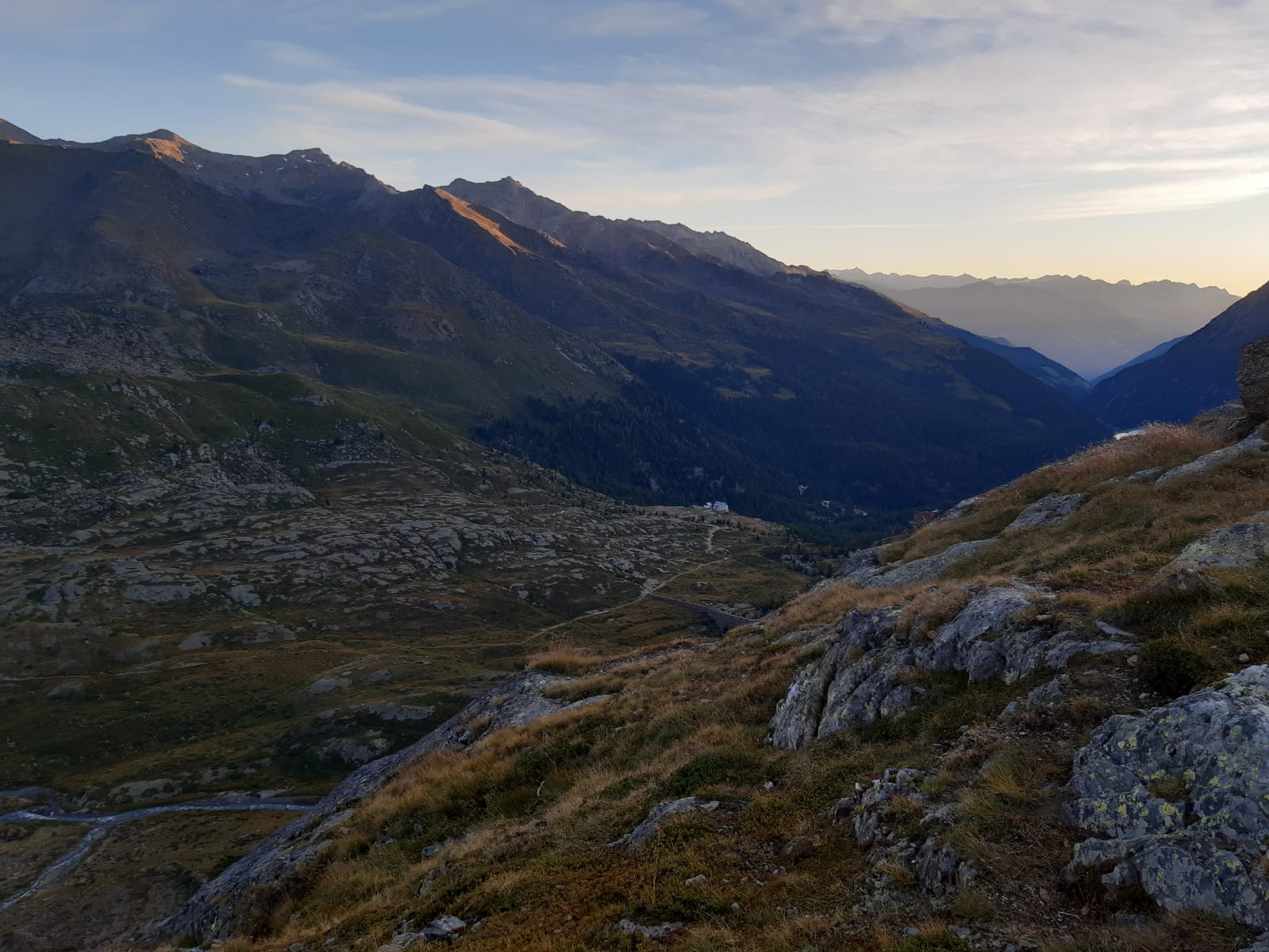
Finstertal + Martelltal + Otzi

Perched high in the mountains of the autonomous region of South Tyrol in the Alps, there sits a mountain hutte where the Mountain Chair of Hydrology, Markus Disse, and his Mighty Wizard Gabriele Chiogna, commune with the Old God Nature (/‘nā-chər/, /’neɪtʃə/, /’nei-chure/).  With the assistance of his guard, Michael Tarantik, Brenda Rubens Venegas and Florentin Hofmeister, they study the language of the mountains, the discussion between the Earth and Water, the jokes between Flora and Fauna, The Poetry writ large in the sky.  I was lucky enough to see this spectacular part of the world during a visit to Germany from Aug 21 to Sep 15, 2020, under a travel arrangement with the Technical University of Munich (TUM) to consider innovative flow methods in alpine streams and assist in the installation and calibration of two AutoSalt systems.  I visited Martelltal and Finstertal with this elite guard, right in the trough of the pandemic waves.  I swear, I didn’t cause the second wave.

Finstertal

[rev_slider alias=”hs-finstertal”]
We installed an AutoSalt on Finstertalbach (bach = brook) in Finstertal (tal = valley) on Aug 25, 2020.  This picturesque little brook is tastefully, almost suspiciously, accompanied by the Zen chime ringing of nearby cow’s bells wandering around the alpine heather. This necessitated a protective electric fence around the installation tank.  Fence safety is demonstrated above by the TUM H&S officer, Michi , observed with great concern by Brenda and Floretin .
Although an ~ 1:30 year flood happened on the Adige River, which joins the Eisack (Isar) River, in nearby Bozen (Bolzano) while I was in town to see to the Iceman (Otzi) exhibit, I did not cause this flood.  Nor did it generate much of an event at the much higher elevation Finstertalbach site.  Monitoring continues at that site.  The flows reached higher levels at the lower elevation Martelltal (see below)

Otzi (the Iceman)

If you don’t know the story of Otzi, I recommend listening to the podcast History on Fire by Danielli Bolleli.  This history professor has a musical accent and an engaging way of telling historical stories that make them relatable and entertaining.  Otzi died in the nearby mountain pass some 5,300 years ago.  Let me write that out so it sinks in: Five Thousand, Three Hundred Years ago, making him the oldest mummy ever found.  Not just a skeleton, but a mummified corpse kept frozen and humid until 1992 when he was spotted by some hikers and dug up.  It’s the scattering of cultural artefacts about his remains, his belongings, his copper axe and half made longbow of exquisite craftsmanship, and the arrowhead buried in his shoulder that make him and his story one of the oldest murder cases in history.   If you are ever in the area, I highly recommend the exhibit.  Book your ticket online to avoid the lineup.  The highlight for me was looking  into our small ancestor’s steady eyes as he watches for his pursuers, and his cool tats.

 

 

 

 

Martelltal

We arrived in the Martelltal on Aug 26 after a placid drive from the Austrian Alps to the Italian Alps.  The TUM students were coming the next day, along with the Enigmatic Wizard Gabriele Chiogna and Doctor of Charm Markus Disse, and so we needed to work fast to ensure everything was up to snuff.  After dropping our things at at the Zufallhütte (actually, the cable car carried our things to the hut and we hiked up as light as feathers) we set to work.  The AutoSalt on the Plima River is a 300 litre Intermediate Bulk Container (IBC) that Florentin and Michi purchased locally.  This tends to be what customers choose rather than ship bulky tanks, stands, and power systems from Canada.  These are 1/2 a standard pallet.  We’ve only found 1000l IBC’s here in North America so far.
Strangely, we found that the AutoSalt had been trying to inject over the last month, but with no record of pulses from the flow meter.  This was a mystery until we removed the hose leading into the river and found everything working but the hose.  It turns out, it was installed so deep in the channel, that the outlet had become covered in finely pack debris which prevented the brine from being injected.  This was quickly remedied and measurements were made overnight.

Sloping-Max Filter

One particular challenge at the downstream sites, shown in Figure 21, is aeration and turbulence, on both the left bank and right bank.  We’ve struggled with aerated signals for years and I think I’ve finally found a filter that preserves the integrity of the source conductivity.  Aeration is not random noise, it only lowers the conductivity.  So the idea with the filter is to lay a filtered signal on top of the aerated signal and

recover the source conductivity.  This appears to be what this filter does.  In the past, I’ve tried a running MAX() filter but this has a tendency to overestimate the area, and thereby underestimate the Q.  The solution was a switch that checks the slope of the line before applying a MAX filter to either the next 5 points (in the case of negative slope) or the previous 5 points (for positive slope).  The excel equation, for row 6, is here: 
=IF(SLOPE(F2:F6,A2:A6)>0,MAX(F2:F6),MAX(F6:F10))
If your ECT data is in column F, for a 5 pt filter.  This particular data is 5s, but your filter size will depend on the amount of aeration, the duration of the pulse, and the sampling interval.

I’ve called this the Sloping-Max filter after a dog, Max, who is skilled at laying down on uneven surfaces and making them look aesthetic.
Good dog, Max .

Figure 23 shows the data on a rising background ECT signal.  It was quite a large fast moving flow and you can see the pump from the AutoSalt almost reaches an equilibrium with the flow (as in constant rate) but we are only interested in the mass conservation.  While it’s not written up, we’ve proven many times that you do not need an instantaneous injection.  You can prove this yourself if you have multiple injections during a site visit with a relatively stable water level.  Compare the individual SDIQs to the SDIQ derived from dividing the total NaCl mass by the the combined area under all breakthrough curves.
After running the above formula on the aerated signal, we came up with this result. Looks reasonable.  Here are some other examples.

Figure 23: Salt Injection on top of natural BGECT Variation after Sloping-Max filtering.

While these results look good, how do we know the area under the curve is conserved?  To test this assumption, I took a several SDIQ records with no aeration and ran it through several versions of the filter, including a 99%ile, 90%ile and 50%ile filter of various sizes.  While not exhaustive by any means, the results, shown in Table, are encouraging.  This table shows that there is no apparent benefit to choosing the Max over the 99%tile.   Both of these filters faired better than the 90%ile and 50%ile.  In fact the Max is the most accurate, which is great because it’s the easiest to implement.  Results worsen as the number of points increases.  5 points seems to be a sweet spot.  The larger kernel size was limited to the first trial.

The LB probe at Plima was far noisier, shown in Figure 25.  The salt pulses were very difficult to differentiate.  We had to use a 20pt sloping max filter and still only 3 SDIQs gave reasonable results compared to 16 SDIQs from the RB probe.  The resulting filtered signals are compared between LB (AT56-Red) and RB (AT57-Blue) in Figure 26.
 

Despite this challenge, we did find relatively good agreement between LB and RB (shown in Figure 26) when the signals were sufficiently strong, and the rating curve generated is shown in Figure 27.  The Hydrograph and the SDIQs are shown in Figure 28.   In this figure, we were on site for the first night and set the system for a high injection rate, hence the higher density sampling.  We didn’t quite capture the peak event on Aug 30th, close to it.  The AutoSalt is now built with a RCVector.csv file with the requested number of measurements per bin.  An examination of the RCVector.csv and the AutoSalt log, together with the code, explains the mystery.  The stage bin from 0.64m to 0.73m had only 2 SDIQs in it, which were spent on the prior events.  While the stage did climb to 0.74m, the AutoSalt checks for a falling stage before injecting.  When the stage had fallen by the required amount (0.05m) it then checks the RCVector. csv again.  By that time, the stage was back within the lower bin with zero remaining SDIQs.
Since this deployment we have changed the code to try to better capture peak events, as well as allowing a Zero DH value (the user is thereby relying on other logic to make injections, such as simply filling the RCVector.csv bins.

TUM Students, Dr. Chiogna, Dr. Disse

Well, the students came on Aug 27th and there was much joy and merriment.  The Wizard Chiogna was indeed a wizard with words and we had a great time (in the evening after delicious dinner and with a few steins of radler and the finest bavarian bier) playing Stadt Land Fluss Game (City Country River), but modified for Hydro-City-Crime.  I’m not going to say who’s idea the latter category was, but it is surprising how many there are (and how many Dr. Chiogna knew) some of which I’m regularly guilty of (wearing plaid on plaid for example).  We played in English, which I was the only native speaker, and somehow I lost every game.  Brenda and Gabriele won every time.  I can’t ‘splain it.  Ain’t fare, that’s fo’sho. (Another great evening game, coincidentally was Wizards.)

Well, the visit was overall a success and is captured in the Quasi-SciFi story Fathomland: The Next Wave .

Conclusions & Recommendations

It’s been a busy year, despite the lockdown and restrictions.  We finally separated Art & Science, not an easy task, but we got ‘er done.  The Cultural Artefacts will make all of our excavation sites more interesting 5,300 years from now.  We recommend you:

1. purchase some Fathom Weights ASAP (alternately purchase a QiQuac or AutoSalt and get the weights FREE!  You too can be a fashionista like Frode from NVE (check out those earrings!) While I’m on the topic of NVE and Frode, look how smart this is.  Geez, I wish I was that smart.
2. read the entire Fathomland Tale, Parts I and II and be sure to listen to the fantastic audio bits.
3. purchase a QiQuac Highlander and receive your FREE t-shirt! (a 42$ value)
4. vote on your favourite Sci-Fi movie and Book for the Alpha (Fe)male Sci-Fi Club.
5. read about that time I went to PNG and discovered a tribe of Neanderthal,  documented by my chum James Wood (aka Craig Sterling)

[efn_note]if you like this, check out some of James’ other military, erotica, and science fiction writing.  You may find hints of Haruki Murakami, Robert Graves, and Paul Bowles as I did, although, I mean, not nearly as good as those authors, but still..[/efn_note]

invite me to come to your country for training and you may find YOUSELF fictionalized in a 2-D caricature of youself in the next Fathomland Tale!

Make your Fathomland Cultural Artefacts purchases today and have a Merry Christmas.
Tschuss.