Cover Image: Fathomland by Fenella Jacquet + Gabe Sentlinger
Fathom Scientific is committed to making your #SaltyLife even sweeter. We’ve done this by creating the Watershed Information Tool (WIT), currently comprised of 9 online tools (Maki Rolls in Figure 0) in the WIT-HM suite.
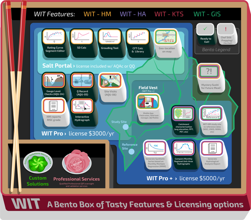
- SD-Calc is an online Salt Dilution Instream Q (SDIQ) processing tool to post-process and manage all SDIQs and CFTs.
- CFT-Calc & Library allows you to calculate the Calibration Factor – Temperature compensated from raw measurement files OR use an average CF.T from site previous site visits. It also tells you the Expected CFT based on Richardson et al.
- Rating Curve Segment Editor (RCSE) is a powerful rating curve development tool to generate Compound Rating Curves based on hydraulic principles, and manage them over the life of a hydrometric station.
- The Grouding Tool is the Grouping + Grading tool to group Salt Dilution injections/flow measurements into a single Group with associated uncertainty and data grade. This tool also allows you to export to Kister’s Wiski or Aquarius Time Series.
- Kronos Time Series (KTS) is a time series database tool that will manage all time-series data, as well as convert your Rating Curve time series to a hydrograph using stage data.
- *NEW The WaFFFling tool is the Water Filtering, Fitting, and Filling tool used to extend the tail of salt dilution measurements, estimate rising limbs, remove artifacts of aeration, and more!
- *NEW The Gauge Level Check (GLC) Tool is ready for testing! This tool tracks the offset between reference stage, datalogger (dl) stage, and generates a Rating Curve (RC) stage from a time varying stage_offset with optional pzf_shift.
- *NEW The Generalized Regression Analysis Tool, Eh?” (GRATE) tool is the beginning of a larger tool to quickly generate regression analyses between channels and fill or create new channels based on the regression. It currently lives in the Modify menu of the Manage Tool
- *NEW KTS-Sink Service This new service in KTS will pull downloaded files from AutoSalt and AQ devices and plot them in near-realtime. Add Modify functions to the uploads, such as an offset.
- *NEW WALLY-GIS for Watershed Delineation and HydroStat estimation. Currently in Beta and operating for the entirety of British Columbia from 7:30 to 17:00 PST. Sign up for an account here.
These tools are the starting point on your journey towards complete hydrometric and hydrological mastery, as presented here . The RCSE and Grouding Tool now handles Salt Dilution measurements as well as imported Bucket, ADCP, or V-A measurements. The KTS currently can import any .csv time series, and is now able to handle live measurements from the AutoSalt telemetry system.
This Sounding gives Ye Traveler of Salty Roads the knowledge to navigate the cavernous depths of the maze towards hydrometric truth, battle the dreaded CF.T monster that lurks at the top of the stairs, win the hand of the handsome and beautiful SDIQ (with contractual Uncertainty) and emerge victorious with the treasures of the Golden Rating Curve. Enter… if… Ye… Dare!
- 1.0 SD Calc
- 1.1 SD Calc Tool Overview
- 1.2 CF.T Tool and Library
- 1.2.1 CF.T Current File
- 1.2.2 CF.T Stored Value
- 1.2.3 CF.T Manual Value
- 1.3 Discharge Calculation
- 1.3.1 3rd U/S Probe Tool
- 1.4 Importing Other Filetypes into the SDCalc
- 1.5 The WaFFFling Tool
- 1.5.1 Basic Idea
- 1.5.2 Remove Aeration/Random Noise
- 1.5.2.1 Aeration Noise
- 1.5.2.2 Random Noise
- 1.5.3 Extend the Tail
- 1.5.4 Extend the Rising Limb
- 1.5.5 Extreme WaFFFling
- 2.0 Rating Curve Segment Editor (RCSE aka Rating Curve Tool)
- 3.0 Grouding Tool
- 4.0 Kronos Time Series
- 5.0 The Gauge Level Check (GLC) Tool
- 6.0 Device Dashboard
- 7.0 Tutorials
- 8.0 Technical Appendix
- 9.0 References
- 10.0 FAQ
1.0 SD Calc
(at salt.fathomscientific.com. Contact us for an account)
(Updated Dec 1, 2022)
The Salt Portal is an online post-processing system to easily load, view, process, grade, and manage your QiQuac and T-HRECS-DL (AT) data. It instantly plots your measurements against a rating curve.
Features:
- Allows Fathom Scientific Ltd. (FSL) to
spyoversee and assist the QiQuac operator with their measurements and troubleshoot some problems remotely. - Allows Organizational QA/QC whereby technicians can upload SD data, and a supervisor can then review and approve measurements, and compare to existing rating curves.
- Export data for import into DataBase Management Systems (DBMS) such as Aquarius Time Series or Kisters Wiski.
- Quickly calculate Q and Uncertainty to all recommended guidelines to achieve a BC Resource Inventory Standards Committee (RISC) Standard Operating Protocol (SOP) Best Practices (BP) grade.
- Rigorous Uncertainty Analysis as per Sentlinger et al (2018)
- CF.T derivation, expectations, and uncertainty as per Richardson et al (2017)
The Tool is currently in Beta and these instructions will eventually be replaced with a more detailed online guide.
- Login to https://salt.fathomscientific.com using login credentials provided by FSL. It may not work behind a corporate firewall or with Microsoft Edge. You can possibly tether your computer to your phone’s data plan if necessary to bypass your corporate firewall. We test on Chrome and Firefox.
- Create a new Project (for example Culliton Creek HPP)
- Create a new Station (for example Culliton Creek DCP)
- If desired, add Station, Visit, or Background photos under the Edit Station view.
- You can also re-assign a Station to a different Project in Edit Station view.
- Upload a new measurement by selecting “Upload & Edit SDIQ File”. SDIQ stands for Salt Dilution Instream Q.
- This should take about 5 seconds for normal QiQuac measurements but can take several minutes for larger AT files spanning several days with 5 second data.
- If the spinning bar at the top stops without the page updating with a graph, then there has been an error. Try again and contact FSL if unsuccessful.
1.1 SD Calc Tool Overview

The Salt Portal is an interface to an underlying database. The database stores the original data file, and relevant CF.T and SDIQ measurement parameters such as mass of salt injected and Start and End times. CF.T records and SDIQ records are independent. This allows the user to select a historical CF.T measurement to apply to the SDIQ measurement. It also allows several CF.T measurements independent of an SDIQ measurement.
When you first upload an SDIQ file, a new record is created every time Save SDIQ or Save CF.T is clicked. In this way it’s possible to process several measurements from the same file sequentially and quickly, for example when processing an AutoSalt T-HRECS-DL file shown in Figure 1.1. The flipside of this functionality is that you cannot Save SDIQ, Edit the same SDIQ, and reSave the same SDIQ: a new record will be created. If you click Save SDIQ, then change the Mass, clicking Save SDIQ again will create a new record.
To Edit a record after saving, you must first exit the tool by clicking Back or on the Station name at the top, then clicking the pencil tool beside the record. When entering the tool from the Edit path, every time you click Save SDIQ or Save CF.T it will overwrite the existing record. However! If you enter the tool from the Edit SDIQ path, the CF.T pointers will not be set properly even though the CF.T used to originally calculate the Discharge will be correct. Clicking Save SDIQ will write over the existing Discharge record, but clicking Save CF.T will create a new CF.T record. Conversely, entering Edit CF.T will overwrite the existing CF.T but Save SDIQ will create a new SDIQ record. Clear as mud? Excellent, read on!
1.2 CF.T Tool and Library
The CF.T is the relationship between [NaCl] and Electrical Conductivity in μS/cm. We use Temperature Compensated EC, or EC.T, or Specific Conductivity, as per the recommendations in Richardson et al. (2017). Following this reference, there are 3 possible CF.T entry methods, each with its own tab in the CF.T tool. Current File (derived in situ), Stored Value (from this station record), or Manual Value. From the abstract of that paper:

The calibration factor can be determined with an uncertainty of less than ± 1% under “best-case” conditions, and the uncertainty may be as high as ± 4% under less favourable conditions. If calibration is not performed, CFT can be estimated from the relation between CFT and background temperature-corrected electrical conductivity (ECBG) with an uncertainty of about ± 2%, or estimated as a set value of 0.486 mg·cm·μS-1·L-1 with an uncertainty of about ± 2.8% for a properly calibrated probe
And from the Draft BC RISC SOP guidelines:
For mass balance methods, the user may derive CFT calibration coefficients either by: i) deriving in situ CFT at time of measurement (preferred); ii) using a site specific, sensor specific CFT derived over multiple measurements; or iii) using the published lab derived constant (Richardson et al. 2017)
Figure 3 shows all CF.T values from Richardson et al.(2017). From this figure, we can see that the average CF.T is around 0.49 mg·cm·μS-1·L-1 with a slight dependence on Background EC.T (1.5% over 500 μS/cm) but this is not a hard rule and the CF.T can be between 0.475 – 0.50 μS/cm over the entire range of Background EC.
The QiQuac and AutoSalt use a default CF.T of 0.486 mg·cm·μS-1·L-1. The expected CF.T is between 0.486 mg·cm·μS-1·L-1 ± 2.8%, which is between 0.474 and 0.500 mg·cm·μS-1·L-1. The Salt Portal will calculate this value + the small Background EC.T dependence. If the R2 falls below 0.98 OR the derived CF.T is <0.4 or >0.6 mg·cm·μS-1·L-1, the CFT report will turn red. When this is the case, the user can choose to use the Expected CF.T with the associated uncertainty (around 2.1%) by selecting “Use Expected CF.T”.
1.2.1 CF.T Current File

- After uploading your file, you will land in the CF.T page, shown in Figure 1.3. The tool will try to automatically determine the placement of the steps of the calibration. This seems to work best for 5 second data with steps of ~10 μS/cm. You can train the CF.T calibration by using the Box Select tool. If this tool does not properly select the steps, then unselect and reselect the calibration with the Box Select tool. When Auto is unselected, then the steps are evenly divided across the selection.
- Enter the correct CF.T Calibration parameters. We ship QiQuac kits with 5.00 g of NaCl in 1.00L of distilled water. The Salt Standard can be checked with another EC.T probe calibrated around 10 mS/cm; it should be 9.03±0.03 mS/cm. Our standard CF.T method is to inject 1.00ml of this standard solution into 1.00L of River H2O.
- To fine-tune the step selection, use the Adjust Calibration Steps sliders. The checkbox informs the tool to adjust all subsequent steps based on the current slider position. Unselect the Link checkbox to prevent this for a given step. Adjust the Calibration Step Slider Sensitivity to increase range of each step slider.
- Examine the CF.T, the R², and the Calibration plot below the calibration sliders to achieve an acceptable CF.T. The CF.T has an acceptable range for a properly calibrated probe, using temperature compensation to 25°C. This is detailed in Richardson et al. Essentially, it’s 0.486 mg·cm·µS-1·L-1 ±2.8% with a small positive relationship on BG ECT. For higher BG ECT, i.e >200 μS/cm, the CF.T could be >0.50 mg·cm·µS-1·L-1, although not necessarily as it depends on the chemistry. Very low conductivity water, i.e. <50 μS/cm should not have a CF.T exceeding 0.50 mg·cm·µS-1·L-1 . The R² should be 1.00 or greater than 0.99
- Once the CF.T is satisfactory, click Save Calibration to create a new CF.T record.
1.2.2 CF.T Stored Value
As per Richardson et al. (2017) it is acceptable to use a site derived CF.T. This may depend on the EC-T calibration of the meter, or the Background EC.T, however. Operator oversight is required when selecting an appropriate CF.T. The uncertainty associated with a stored value is assigned to the selected CF.T and Discharge measurement. To select an appropriate CFT, you can sort the table and select records as appropriate, based on :
- Device
- Background ECT
- Most Recent
- Other
The statistics associated with your selection appear below the plot showing your selection. Select “Use Average” or “Use Selected” to apply the derived CFT to the current measurement.
1.2.3 CF.T Manual Value
If no CF.T available, of if the CF.T is known, it can be entered directly. An uncertainty of 5% is automatically assigned to this method, so it should only be used as a last resort. Using the Expected CF.T has an uncertainty of only 2.1% and should be used instead. If a QQ file is used, the value from the QQ is set as the default.
1.3 Discharge Calculation

Once the CF.T is chosen, the Discharge can be calculated. The Discharge Calculation page, shown in Figure 1.4, is divided into five areas:
- The pulse (aka Breakthrough Curve) selection are showing the box select tool in red.
- The Rating Curve plot (note the Rating Curve Tool button in the upper right).
- Discharge Calculation variables.
- 3rd U/S Probe configuration
- Summary Information. Note that the Calibration Results are used to derive a CFT, but the CFT used in the Discharge record is stored separately from the CFT record.
To begin processing a measurement:
- Enter the mass of NaCl used. This will be populated with the Mass from the Summary line in the QQ File.
- Zoom in on the pulse to better see the shape and Background EC.T.
- Select the pulse using the box select tool. You do not have to select the top of the pulse; the tool only chooses the start and end time from the points selected at the extremities. Also it selects the middle of the start and end ranges.
- You can zoom in on the Pre- and Post- background EC.T to look for any slope or evidence of an incomplete pulse. Currently there is no way to fill in a missing tail, but this ability is on the task list. Fine-Tune the Start and End times using the sliders and sensitivity bar. If all the sliders are at the maximum value and you still need to adjust the start and end time, reselect the data using the box select tool.
- If you believe the Post BG_ECT should be lower (missing tail), the tool offers the ability to enter the BG_ECT manually, or copy the Pre- BG ECT. The tool will assign an appropriate error based on the difference between the EC.T values in the selected range and the manually entered BG ECT.
- The Discharge summary on the right should display results with uncertainty. The function will take the standard error, s, about a regression line trained from the pre- and post- BG ECT values and result in a lower uncertainty. If this is left unchecked, s will be the standard deviation of both pre- and post-BGECT together and result in a higher uncertainty.
- For a good measurement, the uncertainty should be less than ±5%. The uncertainty shown is the 95% confidence interval. If it’s larger than ±5%, check the mass uncertainty and also the CF.T uncertainty.
- Click on the Rating Curve Tool to work on the Rating Curve or the Grading Tool to create a group (CH0 and Ch1 for example) and Grade the measurement, and export to Aquarius Time Series or Kisters Wiski.
1.3.1 3rd U/S Probe Tool
Figure 1.5 Since 2019, QQ’s have the ability to record and compensate using a 3rd U/S sensor. This can be challenging to properly take into account in the field with the QQ, and it is easier to consider in the Salt Portal. The 3rd U/S Probe must be adjusted in 3 dimensions: X or transit time, Y or EC.T Offset, and ω or frequency. While the salt wave has no repeating signal, based on Fourier analysis, any signal can be reconstructed from adding component signals of different frequencies. As it turns out, the U/S signal has more higher frequency components than the D/S signal, in general. It depends on the inputs to the mixing reach. If there is a significant confluence with two different ECT patterns, then this will introduce more higher frequency components into the D/S signal. If there are no significant inputs into the mixing reach, then the D/S signal will be smoothed out by the storage elements in the mixing reach. We have hence named this filter function value, the Smoothing Factor.
- The transit time can be calculated in the field with the QQ by pressing the “Injection” button on the 3rd U/S T-HRECS Radio when making the injection OR by adjusting the Pre-BG ECT for CH2. If the button is pressed, a “-100” is sent and recorded on the EC.T channel. The arrival time is determined by the rise of the ECT as the salt wave passes. This is handled automatically in the QQ.
- The EC.T offset is also handled automatically in the QQ and Salt Portal but lining up the Transit Time adjusted U/S probe signal with the Pre-BG ECT of the D/S channel signal.
- The Smoothing Factor is currently only handled in the Salt Portal. There is no automated method to filter out the higher frequencies in the U/S signal yet.
1.4 Importing Other Filetypes into the SDCalc
The Salt Portal only recognizes QiQuac and T-HRECS-DL file types currently. However, it is possible to both pre-process files (such as remove outliers or correct EC.T for a new temperature) and process records from other devices within spreadsheet programs such as MS Excel. To do so:
- Open the file in Excel, or other spreadsheet software.
- Manipulate the file if needed, but don’t manipulate people, unless required.
- Open a QQ file you know that you can import (or simply download an existing one using the download button from the Station View page.
- Copy and paste in your EC.T data. Don’t worry about the EC,Temp, header, or measurement (i.e. mass, Q) columns.
- This step is important. When you save as .csv in excel, the current date-time format is saved to text. The date-time format must be YYYY-MM-DD hh:mm:ss in order for WIT-HM to recognize it. You can set it to this by formatting the date time column, format->custom->YYYY-MM-DD hh:mm:ss . It must have seconds shown or it will throw a “Zero time step detected” error and fail to load. Excel by default displays timestamps by minute and when this is saved as a csv, the second stamp is lost.
- Save as .csv.
Note that the current version requires a minimum of 40 non-zero time step records.
You should now be able to import your file into the Salt Portal.
1.5 The WaFFFling Tool

The WaFFFling tool is an exciting new tool in your SDCalc Tool Bag. It can be used to:
1. Filter out effects of aeration and data spikes
2. Extend tail of truncated pulses
3. Estimate Rising Limbs of SDIQ pulses
4. Remove Biduk Bumps and other anomalous signal artifacts.
5. Completely fabricate an SDIQ.
and much, much more!
Let’s get started….. now.
1.5.1 Basic Idea
The basic idea is this:
1. Select your SDIQ range in the SDIQ tab, select as close to the start of the pulse rise as possible.
2. Choose the Pre and Post BG EC.T where you estimate the start and end of the pulse to be. If you left site before the pulse reached the post-BGECT baseline, then it might be lower than the last EC.T measurement in your SDIQ. Use the slope of the pre-BGECT as a guide
3. Switch to the WaFFFling tool tab and tweak the model for your range of interest. It doesn’t matter how bad the match is outside of your range of interest, but try to match the slope of your EC.T trend near the end, or start, of your SDIQ.
4. Copy your model results to “Final” and “Save Final”. Switch back to the SDIQ tab and select “WaFFFle DS” to use the Final Model results in your SDIQ calc.
1.5.2 Remove Aeration/Random Noise
There are three kinds of noise that can be present in an SDIQ signal
1. Aeration: the most common indicated by drops in an otherwise stable EC.T.
2. Sensor noise: can be indicative of a faulty wire, a faulty temperature signal, a loose electrode, or faulty electronics due to moisture.
3. Upstream inflow: often appears like 2, sensor noise, but can be isolated when compared to the CF.T signal in calm, isolated water. If the noise only appears in the creek, it is likely due to upstream inflow, which might be subsurface.
If the noise source is 1, then we will use a Sloping Max filter, and if 2 or 3, a Spline filter or a wholesale replacement of the trace.
1.5.2.1 Aeration Noise

When air bubbles appear on the electrode surface, the EC.T drops. This is an intermittent behaviour that appears more strongly during high flows, but can be filtered out to some degree. Previous studies have shown that the sloping max filter can remove aeration with minimal (<1%) impact on the final SDIQ accuracy.
In Figure 1.7 we show a typical storm EC.T signal, with a rising EC.T as the shores are swept clean of salty residue, and then the flow is primarily rainfall runoff (which has a very low EC.T). At around 6am, the aeration becomes a significant factor. This noise can be filtered out using the sloping max filter. To apply a 3pt Sloping-Max filter, select it from the dropdown list, select the number of points in the Kernel. A 3-4pt kernel is good for removing local dropouts with minimal impact to the accuracy of the measurement. A 5pt-9pt kernel is good for removing significant aeration noise, but will impact your measurement more, although previous studies show only a 1.3% impact on known good measurements.


1.5.2.2 Random Noise
Removing either sensor or background EC.T noise is more prone to error since we don’t know the true BG EC.T. Sometimes, noisy data can simply be used as is if the noise is gaussian. The calculated uncertainty from the pre-filtered result should be used for the actual uncertainty in the SDIQ. You could also remove noise by using either the Spline, or one of the Breakthrough Curve models, ie. the SCS curve, to replace all or some of the curve. We will see how to perform this operation in the next section.
1.5.3 Extend the Tail
A good SDIQ is a tension between a very long mixing reach for complete mixing, and a shorter time at site for maximum resource hydrometrician happiness. We’ve developed the WaFFFling tool to assist the Salty Traveller to visit the maximum number of sites in a day while not suffering the slings and errors of truncated tails. For example, on Dec 28, 2023 the author went to site in the dead of winter and wanted to leave after 20mins (classic Fathom MO)

Was the impatient hydrometrician lambasted by his superior? Yes, but for other reasons. In fact the cunning hydrometrician used the WaFFFling tool to extend the tail and achieve a Grade A Result.
First, he selected the available points, then copied the Pre-BGECT to the Post-BGECT field. The WaFFFling tool uses these ranges and values to set the initial model parameters. Then he opened the WaFFFling DS tab to see Figure C. The remainder of his activity is documented in the following figures.


Having transformed his superior’s ire into intrigue, the Superior said unto the Author: “Go, fetch unto me three poor SDIQs and use this…. WaFFFling… tool to repair and redeem them. Seek my audience when you have completed this task. Be gone.
The author quickly scurried from the room, bowing, not making eye contact, and desperately trying to keep a devilish grin from his lips as he ran back to his workstation giggling.
1.5.4 Extend the Rising Limb
Sometimes, you miss the start of an SDIQ pulse. This is less problematic for manual SDIQs, but common for AutoSalt SDIQs using wake-up telemetry. We can also use the WaFFFling tool to extend the rising limb backwards in time.

1.5.5 Extreme WaFFFling
From time to time, Extreme WaFFFling is required. In the following example, a very small amount of Salt was injected from an AutoSalt, there was severe aeration, and we missed the start of the pulse. I have not calculated the uncertainty on this measurement, but it’s for-sure larger than the 4.6% reported in Figure 1.19.

More work is required to properly assess the uncertainty of the WaFFFling tool. If you would like to be part of such a paper, place contact me.
2.0 Rating Curve Segment Editor (RCSE aka Rating Curve Tool)

The RCSE is an interface to a database based on the hydraulic rating curve taken from Handbook of Hydrology (Maidment, 1992) and represents the hydraulic reaction of a smoothly varying channel with increasing stage. Each RC Segment has 4 attributes:
- PZF-The Point of Zero Flow, or the stage when no flow occurs
- Coefficient-Is roughly equal to the channel width by a factor of 2.
- Exponent-Is related to the shape of the channel; 1.67 is closer to a rectangular weir, 2.17 is Parabolic, and 2.67 is Triangular.
- Transition-Most rating curves are compound with a different equation applying to each regime, separated by the Transition. Most are 2 part with a transition at approximately the D90 in the hydraulic control. Some can have 3 parts, such as upstream of a bridge, and in extreme cases 4-5 parts.
- Copy LS to copy the Least Squares or Copy Mahal to copy the Mahalinobis RC Parameters to the form.
- Intersect Next: for compound RCs, use this button to calculate the intersection with the next RC Segment above the current one.
The hydraulic rating curve equation is
Q = C(h + PZF)^N (1)
Where h is the stage value. The PZF is typically a negative value if the Pressure Transducer is below the lowest point in the hydraulic control,
Each Rating Curve can have several RC Segments, and also have a Start Date, a Name, and derived Grade. The Equation is also shown in the upper right. This table can be downloaded from the Station View page.
To aid the user in calculating a valid RC, we calculate two fitting algorithms: Least Squares and Mahalinobis. The linear Least Squares (LS) line solves the N and C values for the stage-discharge pairs, given the PZF. The PZF is taken from Area 1) near the LS and Mahal equations. The LS minimizes the distance between the model (A line in log-log space) and the “Use” points. The Mahalinobis minimizes the uncertainty weighted distance, which is a Maximum Likelihood aka Bayesian solution.
The LS RC and Mahal fits are meant as guides, but do not often suffice to represent the entire range of an RC. For this reason, the RC Tool allows you to select points to “Use” in the LS or Mahal RC Fit. The “Copy LS Values” and “Copy Mahal Values” copies the N, C, and pzf values of the current fit to the current RC Segment.
To re-iterate: points set to “Use” are used in the LS and Mahal fitting algorithms, points selected can be set to “Use”, “Exclude” or “Anomaly”
- Use points are used to fit the LS and Mahal
- Exclude are not, but can be used for other RCs
- Anomalies remain set to Anomaly regardless of the RC selected and are not selectable unless “Anomalies Selectable” is checked.
- Exclusive Use will set all selected points to Use, and all others to Exclude
For each RC, the RCSE will remember the status of each point. Only “Use” points and the most recent RC will be displayed on the Station View page.
To assist in the intelligent selection of points, there are a few tools:
- Uncert. < RC Abs. Error: This tool will select all points that have an uncertainty less than the absolute error against their applicable Rating Cure. The “Applicable Rating Curve” is the one residing in the time period for which the point was collected.
- Applicable to Current RC: This tool will select all points that fall in the epoch of the currently selected RC.
- Anomalies Selectable: This toggle will determine if points labeled as “Anomalous” will be part of the selection or not.
- Only Quick Select “Use”: will limit the points selected to those set to “Use”.
2.1 RCSE Legend
There are 7 series in the legend:
- Anomaly: These are points the user has classified as Anomalous. They would not be used in the final RC Grade and also not selected, unless “Anomalies Selectable” is engaged.
- Excluded: Are points currently turned off for RC fitting but still used in the final RC Grade.
- Used: are points used in the current RC fitting and the final RC Grade.
- Bold Dashed RC: is the currently selected Rating Curve.
- Coloured Dashed RC: are the other station Rating Curves.
- LS RC: is the Least Squares fit to the points currently Used.
- Mahal RC: is the Mahalinobis fit to the points currently Used.
The legends in the plot are interactive. Click on a series to turn its display on or off. This is cool.
3.0 Grouding Tool
3.1 Explanation of Tool Name
Grouping + Grading = “Grouding” Tool, obviously.
3.2 Tool Overview
There’s a new tool on the block, and nope, it’s not me. It’s the Grouping + Grading or, as the kids say, the Grouding tool. The idea is that each flow measurement is a pair, or group, of individual SDIQs, each with their own uncertainty and a conglomerate uncertainty. The Grouding tool also adds the 3rd U/S probe signal to the group. Here’s how it works.


In Figure 1, we see several measurements for the Aberdeen Project (Site) and the Pretty River Station. Only 2 channel measurements are currently shown.
The Grading Tool reads the SDIQ from each record, along with SDIQ Uncertainty and displays these values in the upper right. The colour scheme is Orange: Grade C, Blue: Grade B, and Green: Grade A. Only the first Group selected will be graded.
the Q Uncertainty is the Maximum of the individual Q Uncertainty, or DQ:
Q Uncert = Max (DQ, Q Uncert. CH0, Q Uncert. CH1)
for two channels, for example. DQ is calculated as:

The grade assignment is based on :
<7%: Grade A
<15%: Grade B
>15%: Grade C
Only 1 Channel: Grade N
These Grading Thresholds are the default values in the QiQuac and the RISC guidelines here in BC, Canada, Canada. Future iterations of the Salt Portal will have user defined thresholds.
3.3 Measurements
The Measurements table contains all those measurements associated with this Project-Site. Click on a measurements check box to plot it. The colour scheme is always Blue: First series, Red: Second Series, Green: Third Series. If you’d like to plot a group, you must deselect the measurements already plotted. The first three series selected will always be plotted.
3.4 Groups
To manually create a group, select all those measurements that belong to it and click “Create Group”. Alternately, click “Find Groups” to select all those measurements that have a start time within 30 mins of one another and create a group. The 30 min default can be changed in the settings file (eventually). To Export one or several groups to WISKI: BIBER, select them and click “Export Group” The xml file will be downloaded to the download directory. To Delete one or several groups, select them and click “Delete Group”. Groups are very ephemral; don’t worry too much about deleting them. They can fairly quickly be generated again, as they are just pointers to the SDIQ measurements.
4.0 Kronos Time Series

4.1 Overview
The Kronos Time Series (KTS) tool was designed to assist the hydrographer in managing, viewing, and making decisions based on their time series data. It has several Modules, currently being:
- Upload: This Module allows the user to upload .csv files, which must have a DateTime channel and at least one data channel. It contains several default parameter types such as Discharge (cms) and Level (m). File Templates can be saved, along with default Fathom type formats. New data can be used to create a new channel, or add to an existing channel. NOTE: Currently existing data will take precendence where there is an overlap of data. In the future, the user will be given a choice of overwriting or retaining.
- Plot: This is the landing page for the KTS and shows the last displayed plot. Zooming, panning, selecting, and changing displayed channels is easy and intuitive. Take a screen capture or download the image for your reporting.
- Stage-Discharge: Use this Module to convert your station’s Rating Curves to a Hydrograph using a selected Stage record. Does all the heavy-lifting of determining which rating curve and rating curve segment to use for a particular stage and DateTime range. Also allows the user to populate the DL Stage field in MSMTs
- WQMM: is the Water Quality Mixing Model. It was developed by Gabe Sentlinger in 2018 and employed at several hydropower and mining sites. It uses the Constant Rate Injection method to calculate flow downstream of a mixing reach at confluences.
- Manage: This Module allows you to rename, recharacterize, modify, and revert to a previous version. The current stable version has a limited range of operations, but represents the most common data operations. It will continue to expand with time and users.
- Resample: This Module is for resampling all channels in the Time Series to a common time base, except Discrete Series. For example, the T-HRECS DL often logs at 5s, but we may want to view all data in 15min intervals. You can upload all your data first, and then resample OR, select “Automatic Resample” to always resample to the established timebase when uploading. NOTE: The current stable version of the KTS has a limit of 1,000,000 rows per channel. The Time Series Table may take too long to load with more records, so please resample your data if it is approaching this threshold.
- Download: Having your data at your fingertips is nice, fo’sho’, but saving your data in case of service loss, or other mishap is critical for responsible data stewardship. Use this Modeul to download the current instance of all your channels for this Time Series Table. This is also a convenient way to manipulate your data in ways that the KTS cannot, such as merging channels, adding or deleting discrete measurements. Simply download the .csv, manipulate in your favourite spreadsheet or Python, R, etc, and re-upload.
4.2 Working with the Plot Module
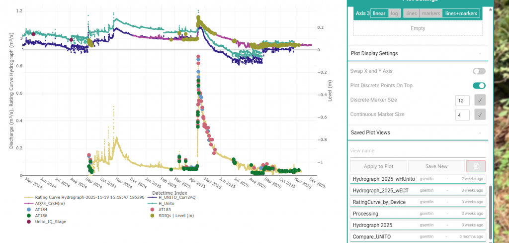
The Plot Module is where most decision making and reporting is done. NOTE: Currently, the last set of channels plotted will be remembered. It’s possible to save your current display parameters such as x and y axes, and plotted channels by scrolling to the bottom of the plot selection panel on the right, entering a plot name, and hitting “Save Plot”. The plot will be remembered in the database. If a plot series is deleted, it will simply be removed from the save plot.
To plot Dependent Variable Channels to the primary y-axis, drag that channel to the Axis 1 box, or double click the channel. Similarly, drag that channel to Axis 2 or back to the Dependent Variable Channels Hidden box.


To incorporate plots into your reporting, either Download the plot as a png, using the Camera tool above the plot, or take a snapshot in your OS. We paste this plot into a formatted chart worksheet in Excel and add commentary, a title block, date/time and version numbers, but you can do whatever the heck you want. We are not the boss of you.
4.3 The Manage Tool
The Manage Tool allows you to Edit your channel name and type, Modify your data, and check its Modification History.
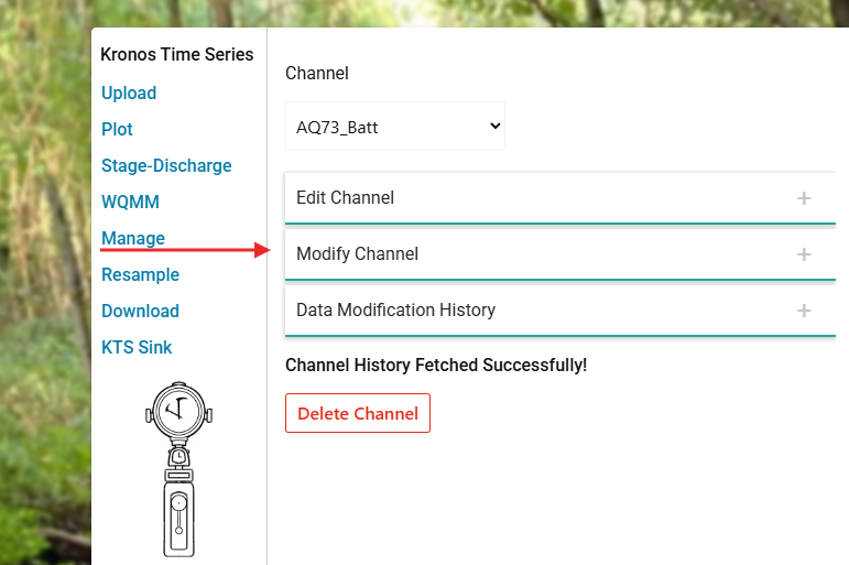
4.3.1 The Edit Channel Module
The Edit Channel allows the user to change the name and type of an existing channel. The “Discrete Series” toggle will change how the channel is displayed, governed by the controls in the right hand control panel, shown below.
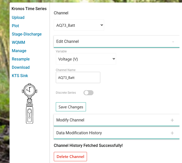
4.3.2 The Modify Channel Module
The Modify module is home to your favourite Modify functions, like Add Value! and it’s evil twin Subtract Value (boo!), the plucky Multiply Value, or the fiendish Divide Value. If working with channels is your fetish, try the Add, Subtract, Multiply and Divide Channels!
*Remember: the target and proxy channels must have the same timestamp, so head on over to Resample beforehand.
*Also Remember: currently the TimeScale DB upgrade manages large timeseries (>25,000) by resampling for the KTS frontend. This can result in incongruent timestamps. If you original data is 15min, and 100,000 rows, you might get 1:00 resampling. Another channel may only have 75,000 rows and be resampled to 0:45. The data will only align every 4 hours. To get an accurate regression, you must Fetch Full-Res data from the right hand panel beneath the channel selection panel (see Section 4.4 below). However, if a regression every 4 hours is sufficient to develop a relationship, when you hit “Apply Modification” it will apply the slope and intercept to the entire range in the backend.
For each of the algebra operations, you can select a range of time to apply to. This can be entered manually into the date-time fields, or selected with the box select tool or the lasso select tool.
NOW! available is the option to append a modify operation to a KTS Sink Service. This is currently only for incoming AQ and AT data stored in the Fathom S3 bucket (available from Device Dashboard > Files) that have been setup with a KTS Sink Service within KTS.
Beyond algebra, there are tools to perform Filter Value, Filter Time, Linear Interpolation, and Linear Regression. In each tool, use the box or lasso select to set the date range over which we apply the filter or linear interpolation. You can manually adjust the range in the date time fields. For all tools, you can use the plot tools to zoom, label, or turn off/on series.
The Linear Regression tool is the beginning of a Generalized Regression Analysis Tool, Eh? (GRATE) a made in Canada regression tool. The first selection is the proxy channel. The Target Channel is the Dependent Variable, while the Proxy Channel is the Independent Variable, or Predictor Variable.
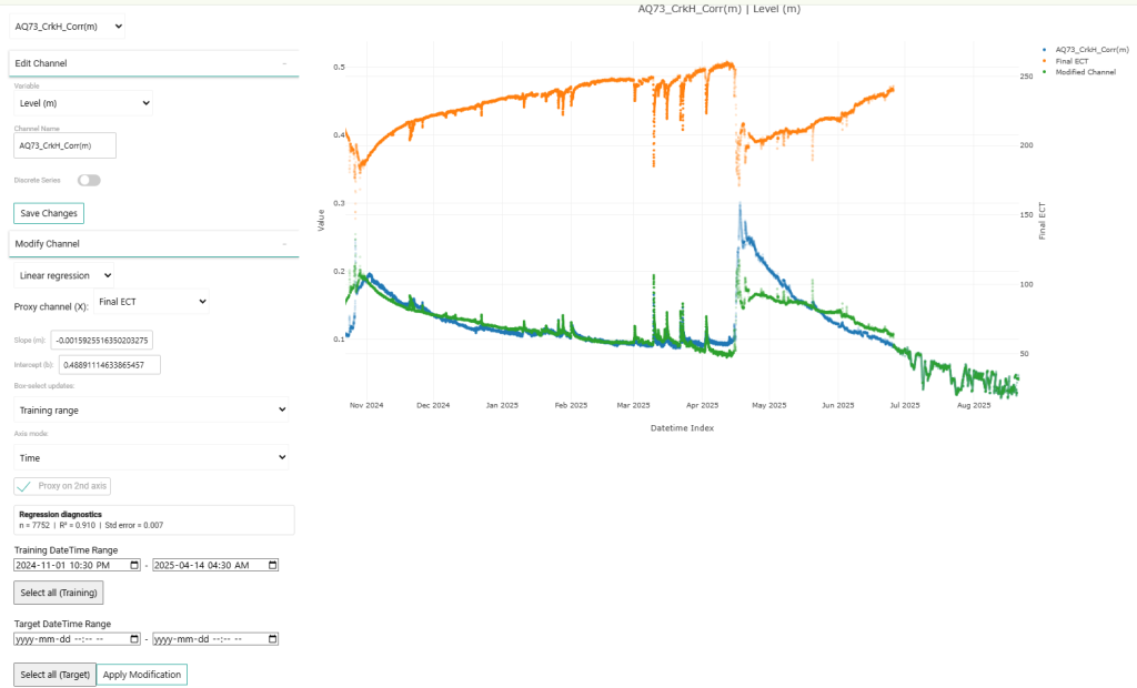
The Slope (m) and Intercept (b) are the next fields that will be auto-populated when you select a concurrent range between the proxy and target channels. These are corollary to the n, R2, and Std Error values. If you change the slope and intercept, the R2 and Std Error will be updated. The Std Error is in units of Target Channel.
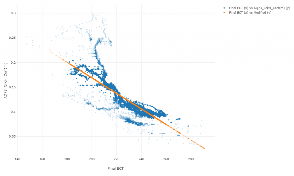
The Box Select Updates dropdown list selects the Training Range, Target Range, or Both. The Axis Mode selects Time or Proxy as X to generate a scatter plot. Within the scatter plot you can select clouds of points to generate your regression analysis, even if they are not sequential in time.
Chose Proxy on 2nd Axis if you have a much different range for your proxy values than your target range, such as depth and EC.T. When you are happy with your regression and target range, select Apply Modification to send the requested change to the Time Series Database.
4.3.3 Data Modification History
This record shows data modification history, with the option to copy or revert the current channel back to historical copy. A prompt will ask if you would like to copy the channel before the modification or afterwards. Just answer honestly.
4.3.2 KTS Sink Service
The KTS Sink Service is a server-side, recurring operation to find all files associated with a given device (AQ, AT, and QQ) and populate a channel within KTS. This is useful for monitoring AutoSalt systems in near realtime. The minimum sink interval is 15mins, and most AQ devices sync to the server every 360minutes if connected continuously, or once per day if on a low-light timer.
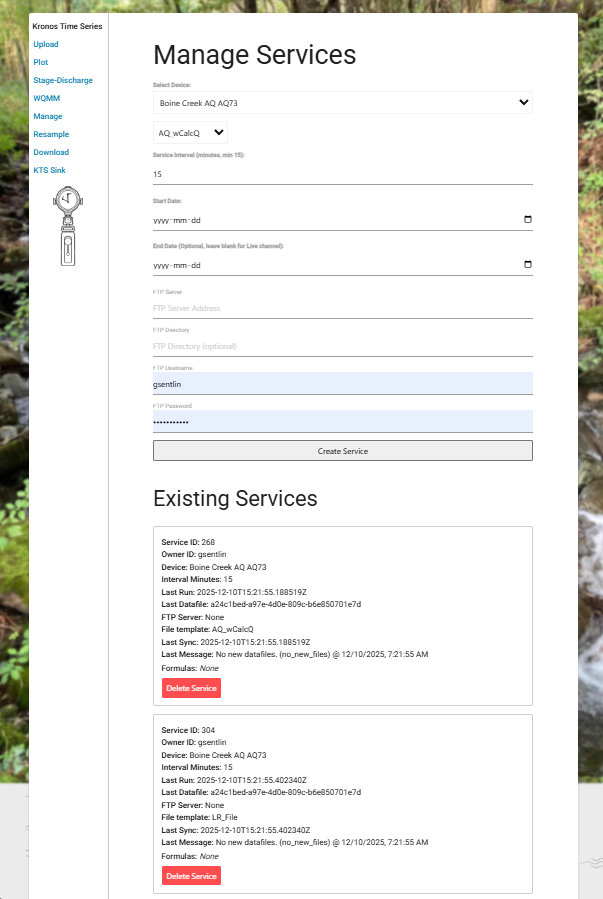
It’s possible to create an FTP service associated with the KTS-Sink service. This allows the user to send channel data to an external FTP server. It’s also possible to add a Modify operation onto KTS-Sink services, such as adding an offset, or slope and offset.
4.3.3 Resample
The Resampling module allows you to resample to a common time step, such as 15mins or daily.
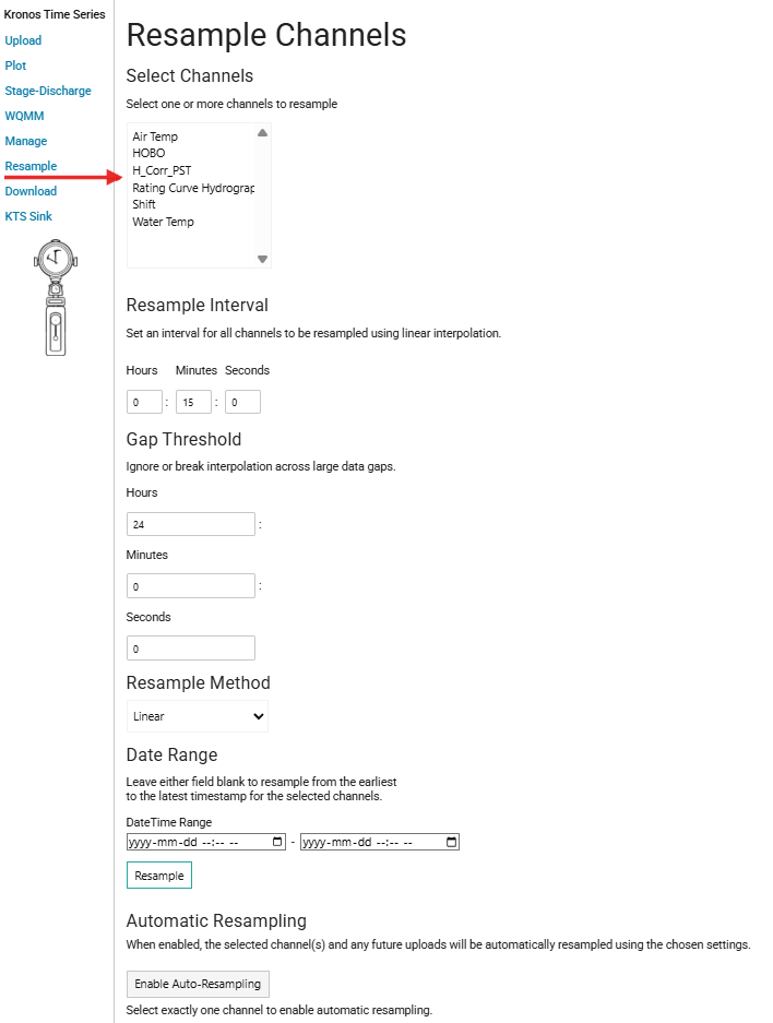
NOTE: In order to speed loading and display, the KTS will appear to resample your data, but it’s simply sampling a subset of your data for display. This is handled in the right hand panel when clicking “Full-Res.” See Section 4.6 Full Res Panel
4.4 Full Res Panel
There is a functional limit to what the KTS can display. We resample the underlying datasets to optimize the user experience. This may not be immediately obvious, but if you go into the Full-Res panel by clicking the button above the plotting panel on the right hand side, you’ll see a list of all the channels and their record count. If the channel contains less than 25,000 records, the entire channel is loaded and displayed. If more records exist, the channel is resampled at a regular interval to stay below 25,000. The user can chose to display all channel records, but will not be able to manipulate the records, simply display them in the current plot windows.
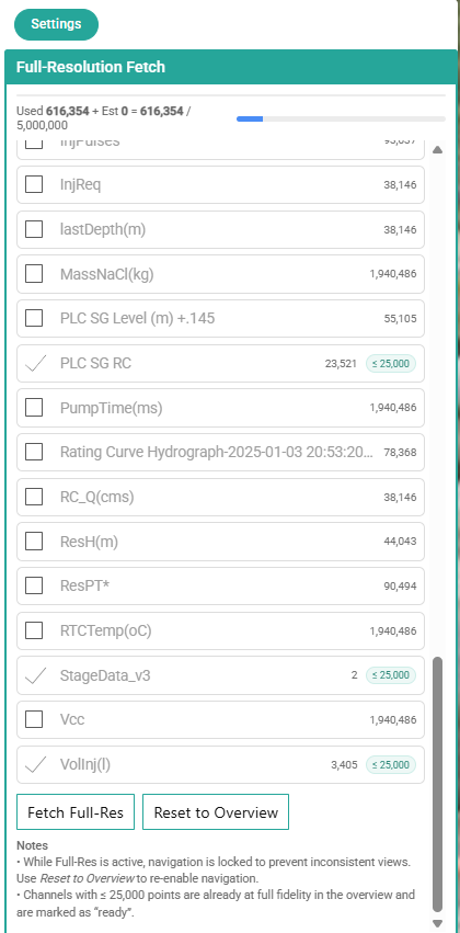
Reset to Overview to restore full functionality of the KTS. The handling of large datasets will be improved in future releases.
5.0 The Gauge Level Check (GLC) Tool
5.0 Overview
The Gauge Level Check (GLC) Tool represents the latest excursion of Fathom Executive into the dark waters of hydrometric data management. This tool manages the relationship between Reference Stage (ie Staff Gauge, or Dipping Point, or BM to WL), the DataLogger (DL) stage, and what is used for the Rating Curve (RC) stage. It’s flexible in that it allows the user to choose what to use for the RC Stage, and provides a buffer between the user’s scratchpad (GLC Table) and that used in the Rating Curve (MSMT Table). It’s important to understand the relationship between GLCs and MSMTs.

The GLC table inherits the attributes and functions from MSMT table, BUT it can be a standalone GLC, or inherit the properties of an existing MSMT. It is always a new record in the MSMT table though. Like V-A, or ADCP measurements, GLCs are a special kind of MSMT with additional fields such as “stage_offset” and “pzf_shift”. Both tables have the fields DL_Stage, REF_Stage, and RC_Stage or simply Stage. The reason for the redundancy is two-fold: 1. this provides a level of backup of site notes and 2. to better represent the field visit model. For example, a technician can visit a site without collecting a flow measurements, simply a GLC check. The user can take a flow measurement at one time, and perform the GLC check at a later time, for example an hour later. The structure of the database allows for both situations. One thing to note: The KTS does not like it when the same date-time stamp (yyyy-mm-dd hh:mm:ss) exists for two MSMTs. For this reason, we add 1 minute if the user creates a GLC from an existing MSMT. The Find New Visits function searches for “unique” site visits. This is arbitrarily set to 240mins right now, but will allow the user to set what constitutes a site visit in future iterations. A screen capture of the tool, in GLCEditor mode, is shown in Figure 6.1.

If you ever find the GLC Tool unresponsive, simply refresh the page; the server may have been disconnected. Like the RCSE and SDCalc, you must have the webbrowser tab selected for the tool to load.

Note: Almost all functions in the GLC tool require either MSMTs or GLCs to be selected. Nothing may happen if there is nothing selected and a button is pressed. Watch for the rotating progress bar at the top of the tool to indicate the server performing the requested action. Starting with a station that has existing measurements, the procedure to generate a GLC Correction Vector and to correct/shift a stage record is as follows:
- Upload your uncorrected, atmospherically compensated stage record to a KTS Channel (see Section 4.1 above.
- In KTS, select the Stage-Discharge button, then select the level channel, then Populate DL Stage. This will take several seconds or minutes depending on the size of the level channel.
- Open the GLC tool for this station.
- Select the channel used to generate the DL_Stage from the dropdown list above the GLC TS Plot and hit “Apply”.
- Quick Populate MSMTs by copying “RC Stage–> Ref”
- Click “Find New Visits”. This will select the MSMTs that have at least 240mins between them (this will be user definable in the future).
- Click the “MSMT –> GLC” button to create GLCs from the selected MSMTs. The GLC Table should become populated.
- Select all GLCs by clicking the top checkbox and click “Delta –> Offset”. This will calculate the Ref_Stage – DL_Stage delta, and copy that value to “Stage_Offset”. You should now see several series in the GLC TS Plot:
- Make adjustments, verify ref stage values, and choose offsets if required.
- Download all the GLCs using the “Download” Button above the GLC Table.
- Back in KTS, upload the GLC table.
- When your channels are ready, click the “Resample” Button and choose your desired interval, usually 15mins.
- Now the GLC table will be converted to a GLC vector with an interpolated point every 15mins.
- Select “Manage” and select your source level channel. In the “Data Modification History” make a copy of the channel. You may wish to retain the original level channel, so you can also copy the channel prior to resampling.
- With either your new copy, or the original file, select Modify Channel, Add Channel and select the GLC vector channel. You should see a rendition of the Modified Channel in the plot on the right. When you are satisfied with the modification, click Apply Modification. You will have to wait several minutes for the change to be affected in the backend database. When the operation is finished, it will display the message “Modification Succesful”. Rename this channel “Level_Corrected” or as you wish.
- Back in the GLC tool refresh the page to see the new channel list. Select the “Level Corrected” channel and Apply. You should now see the corrected vector pass through all your reference stage values if the operation was successful.
- Repeat as necessary and/or open a beer to celebrate.
5.1 Quick Calculate GLCs

Use this tool to complete bulk changes to the GLCs. Note that the GLC Tool does not autmatically calculate values like Delta Stage; the user must enter the value and save it, or use this Quick Calculate GLC tool
- Bulk Set Offset: This function with use the “GLC Stage Offset” value to set the stage_offset for all selected GLCs, and then calculate the new Deltas, as per..
- Calc Deltas: This function will calculate the Pre-Stage Delta (stage_delta = ref_stage – dl_stage) the Total Correction (total_corr = stage_offset + pzf_shift), the RC Stage (stage = dl_stage + stage_offset + pzf_shift) and the Post-Stage Delta (post_stage_delta = ref_stage – stage)
- Delta –> Offset: This function will first calculate the Pre-Stage Delta, then copy that value to the Stage Offset for selected GLCs. It will then calculate and save new Deltas as per above.
5.2 Quick Populate MSMTs

Use the Quick Populate MSMTs function to copy values between fields in the MSMT table. Remember you can quickly make GLCs from existing MSMTs. Often there will be two or more MSMTs per field visit where only 1 GLC occurred. For this reason, we’ve added the Find New Visits function. This currently will find all unique MSMTs with a date time stamp greater than 240 mins (4 hours). Before creating GLCs from sites visits, you should populate the stage fields in the MSMTs
- In the KTS, run Stage-Discharge –> Populate DL Stage. The table on the left, the MSMT table, will show NaN in the dl_stage column until this step is taken. Refresh the page to update the MSMST table.
- In many cases, the “stage” aka “rc_stage” will be the “ref_stage” value, or the staff gauge value. If this is the case, click “RC Stage –> Ref” to populate the “ref_stage” with “stage” values.
- Click Find New Visits.
If all went according to plan, you should see fully populated table on the left (values in ref_stage, stage, and dl_stage) and only unique visits selected. If you wish to add or remove site visits, simply click the checkbox beside each MSMT. When you’re ready to create your GLCs, go to the next section
5.3 MSMT Series <–> GLC Selection

The MSMT <–> GLC tool allows you to migrate MSMTs to new GLCs, and GLC values back to the appropriate measurements. Only MSMTs can be used to generate Rating Curves. This paradigm may change in future iterations of the WIT.
- To quickly create new GLCs based on the selected MSMTs, usually from the Find New Visits function above, click the MSMT –> GLC button. This creates new GLCs from each selected MSMT and adds 1 minute to the date time stamp (since no two MSMTs should have the same date time)
- Add additional GLCs with the “New GLC” function
- Delete GLCs will delete selected GLCs from the table below.
- On the left are plotting options. The RC Plot on the left shows MSMTs RC Stage vs Q. If you select DL Stage and Apply, the RC Plot will show the dl_stage vs Q. Remember for the MSMT table to reflect changes to the GLCS, you must click the MSMT <– GLC button. Likewise for the “Ref Stage” radio button.
- the MSMT <– GLC button will again use the 240min nominal interval and set all MSMTs that have a date time within 240mins to the stage values (dl_stage, ref_stage, stage) from the corresponding and selected GLCs.
- The Log-Log Axes simply sets the two axes to log-log using the pzf of the selected rating curve.
5.4 GLC Editor Panel

Clicking the GLC Editor dropdown will present you with an array of all available GLCs, with the option to add a new GLC. Select the GLC you wish to edit based on the datetime.
The GLC Editor Panel allows the user to edit all parts of the GLC. It allows you to calculate the Pre-Offset Δ, but does not save it, calculates the RC Stage, but you can edit it, and calculates the Post-Off+Shift Δ. It’s intended to be helpful, but flexible.
- Watch Time: is the time recorded in the field data sheet. It’s often local, daylight savings time, but not necessarily. Like the next field..
- Watch Zone: the intent to make the user aware of time zones for better management. Future iterations will take into account the Watch-DL Time stamps.
- Ref Stage: is the water level of the reference stage, above the site datum (zero elevation). Often this is a surveyed staff gauge, but can be a distance between a dipping point (benchmark) over the water, or surveyed water level.
- DL Stage: is the DataLogger stage. This often can fluctuate with respect to the reference stage. Typically this is populated using the KTS-Stage Discharge-Populate DL Stage function.
- Stage Offset: is the desired Offset to apply to the DL stage to achieve something close to the Ref Stage. It need no be the Pre-Offset Δ, but is often close to it. This is because wave action can confound the Ref Stage reading, and the PT Elevation should remain fairly constant between visits if all is stable. It is typical to enter the Ref Stage and DL Stage, Calc Delta and enter the resulting Pre-Offset Δ into the Stage Offset field, then hit Calc Delta again to get the resulting RC Stage
- RC Stage: This can be whatever the user wishes, but is most typically equal to the DL Stage + Stage Offset + PZF Shift. This is what is calculated when you push Calc Delta.
- Pre-Offset Δ: is the Ref Stage – DL Stage. It is prior to the Offset.
- Post-Stage Δ: is the difference between the Ref Stage and the RC Stage. This should typically be close to zero, but if there is a PZF Shift applied, will not be zero.
- PZF Shift: is the artificial increase or decrease of the Point of Zero Flow elevation to match the existing rating curve. It typically changes linearly over time due to environmental factors such as beaver activity, snow-ice backwater, or degradation and aggradation of the hydraulic control, It is the offset applied to the corrected water level in order to fit the stage-discharge point to the existing rating curve. It should be considered temporary, but is useful for achieving reasonable RC Q values in challenging hydraulic controls.
5.5 GLC Time Series Plot

The Time Series plots shows your key GLC variables and how they change over time. You can also select any channel designated as “Level” from the station’s Time Series. It is common to start with your atmospherically compensated, un-corrected DL stage. After you’ve applied the GLC corrections, you can then compare your RC Stage to the final “Corrected” Stage level.
In the figure above, we compare the compensated, un-corrected DL Stage to the RC Stage, the DL Stage, the Ref Stage. The DL Stage should match the time series at each point. See how the Ref Stage departs from the DL Stage over time. If the PT is secure, the Offset should remain constant across time. Slopes, “sawtooth” effects in the “Offset-Line” series should be avoided and investigated. For example, there is an unexplained slope in the offset-line from installation in 2018 to the second site visit in early 2019. There is no obvious jump in the stage record indicating a falling PT (a falling PT would result in an increase in the Offset). The sloping offset-line in early 2021 is simply the time between removal and re-installation of the PT and not a cause for concern.
In most cases, the RC Stage should match the Ref Stage (the orange dot should be within the blue dot). This is the case for the entire record except the last point in August 2024. A small sand-bar at the outlet of the PT pool, comprised of organic material, had collected sand and cobble over the course of the year. We removed the sand-bar during the August site visit, but have added a PZF Shift of -0.07 to the GLC to simulate a linearly increasing rise in the PZF between site visits. This allows the August 2024 Stage-Discharge point to fall onto the established RC, and is temporary because we removed the sand-bar. In the figure below, we show the final stage record ready for conversion to RC Hydrograph.

5.6 Next Steps
Once you are satisfied with the GLC Tools, you can download them by clicking the download arrow next to the GLC Table below the Time Series plot. You can paste this csv into your favourite spreadsheet program and format it, derive stats, and publish. To correct the DL Stage record and generate the RC Hydrograph, still a few steps remain:
- Download the GLC Table.
- Enter the Kronos Time Series where the compensated, un-corrected DL Stage resides and “Upload” the GLC Table Total Corr (m) column.
- If not automatically resampled, you must resample this series to the same time-step as the DL Stage record. This action will create a large vector with a value for each DL time step.
- In the Manage tool within KTS, select the DL Stage record and then Data Modification History. Select the current version and Copy it. Under Edit, rename this new channel “DL Stage_Corr” or whatever you wish.
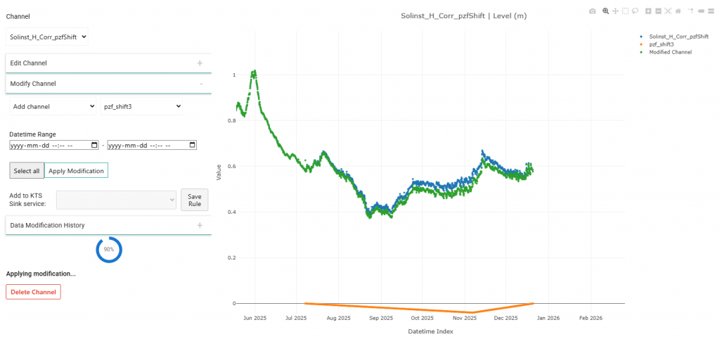
- Select the new copy and Modify Channel > Add Channel and select the resampled Total Corr channel. You should see a preview of the final channel. If all has gone according to plan, you should see something like this figure:

If the preview looks reasonable, then click “Apply Modification” and wait. Depending on the dataset size, it may take several minutes to modify the backend database and resend the final version back to the frontend. You may leave the page once you click “Apply Modification” and the server will work behind the scenes to undertake your bidding.
It’s also possible to apply a pzf shift correction. This is done when there is an artificial hydraulic control change, such as by a beaver dam. In the image below, a 4cm reduction of stage was applied to coincide with the peak beaver activity. The 4cm was chosen to drop the measured Q point onto the existing rating curve.
6.0 Device Dashboard
The Device Dashboard is a way for Fathom customers and crew to access device files, connectivity, and history. This will eventually include repair and warranty status, along with firmware upgrades and recommended service intervals.
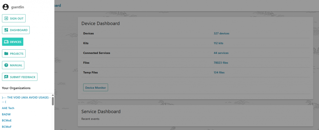
6.1 Devices
The devices page shows all devices currently associated with your organization.
6.2 Kits
The kits shows all associated devices within a kit.
6.3 Connected Services
Connected services are those Kits (AutoSalt only currently) that are connected to the internet and our VPN.
6.4 Files
This page shows all files associated with your devices, the last modification timestamp, and the upload timestamp. These files are stored in the S3 Data Repository and not necessarily processed as an SDIQ or a KTS Channel. You can click on any individual file and download it. If you select multiple files to download, a temporary file will be created.
6.5 Temp Files
If you select multiple files to download, a temporary zip file will be generated to download.
6.6 Device Monitor
The Device Monitor stores device status of those systems connected to our VPN and the internet.

7.0 Tutorials
The following shows several examples of how to work within the WIT-HM tools. These datasets are available upon request, but we encourage you to try your own data. Feel free to contact us at info@fathomscientific.com for assistance or positive affirmation.
7.1 Rating Curve Segment Editor (RCSE) Tutorials
The RC Tool is a powerful and hydraulically valid Rating Curve development tool. There are many ways to select and manage points for your rating curve. We will start with a single compound RC, then work on multiple RCs that change over time. Currently, the RC Tool only works with Salt Dilution Instream Qs (SDIQs) but in the near future (2023) we will allow the user to import any kind of flow measurement.
7.1.1 Example 1. Single Compound RC: Rollergate Channel near Dunedin, NZ

The RC Tool is a powerful and hydraulically valid Rating Curve development tool. Each time a change is made to the models, an “I’m Thinking! Get off my Back” infinite improbability bar will appear at the top of your browser. Wait until this disappears before proceeding.
- To begin, select all points and click “Use” then “Apply”. All points should become blue.
- Now we must exclude the anomalies and invalid points. These are points with a stage or Q of Zero. In this case, I’m going to exclude all the points that are far away from a single RC. We do this by selecting anomalous points with the select tool (use the Shift key for a multi-part selection) and selecting “Anomaly” and then “Apply”. After a moment, those point will become grey.
- The Mahal and LS Fit RC models will update and should generally follow the points, as in Figure 5.1. However, it is clear from this figure, that there is a sharp transition. Rollergate is an artificial channel, shown in Figure 5.2, with steep sides above a stage of 0.55m. This is consistent with a sharp transition at this level.
- To create an RC Segment for the lower portion, select all those points above 0.55 and then select the “Exclude” radio button, then Apply. Both the red LS RC and green Mahal series should pass through just the lower portion of the curve, shown in Figure 5.3. Adjust the LS and Mahal pzf (beside their red and green equations) until the C and N values are reasonable (see Rating Curve Segment Editor (RCSE) above for reasonable values).
- When you are satisfied with the RC segment, it’s time to update the RC Segment record. To do so, click on the drop down list called “Rating Curve Segments” and select the first segment. Enter 0.55 into transition. Click “Copy LS Values” or “Copy Mahal Values” to copy the values from the model into the fields for this segment. The RC Segment record will be updated. Close the form.
- To create the upper RC, click on “Select RC Segment” and “Add new segment”. A generic RCS form will appear. Click “Swap Use/Excl” to swap the excluded points from lower to upper. Set the LS/Mahal pzf to +0.2 (meaning the outlet of the hydraulic control is below the PT). Populate the new segment with LS or Mahal values and save it to the database by clicking “Create”
- Select all points and set to “Use.” Because they are labeled “Anomalous” using the box select will ignore the anomalies.
- The Station Grade should be A with 80 points and an average error of 4.36%. Because there is currently only 1 RC, the RC Grade will be the same. As more RCs are added to the Station, the Station Grade will change based on the average error between the measurements and their “Applicable RC.” The “Applicable RC” is that covering the time epoch in which the measurement was made. It IS possible to USE measurements from outside the RC Epoch, for example for very large or very small measurements, but their error will only be counted against the Applicable RC.


7.1.2 Multiple Compound RC: Noosgulch Creek in Bella Coola, B.C. Canada
Noosgulch Creek in the Bella Coola valley is the traditional territory of the Nuxalk Nation. From their website: “Guided by Nuxalk knowledge, tradition, and protocol, the Clean Energy Department is committed to energy sovereignty in Nuxalk territory through clean energy projects that enhance quality of life and protect the natural environment.” The nation is looking to offset some of the 3million litres of diesel used to provide reliable power to the Bella Coola valley, while still maintaining environmental and financial sustainability.
This project uses the AutoSalt system coupled with the Unidata NRT Satellite Telemetry system to collect high frequency flow measurements. To date, there have been 136 SDIQs, used to develop 3 rating curves over the course of 9 months. We’ll start will all data in the RC Tool.

The first step is to look for trends in the SDIQs. We do this by stepping through time. First sort the SDIQs from oldest to newest by clicking on the “Date” column. Select the checkbox beside the first SDIQ. Continue to add to your selection by pressing Shift and the Down arrow on your keyboard. You will see selected SDIQs become orange as they are selected. There is a jump to a second cluster of SDIQs starting May 9, 2022. Push Shift Up to de-select May 9. These measurements will be the training data for your first rating curve. Click “Swap Selected” to select all measurements other than your selected. Next click “Exclude” and “Apply”. Now only your first RC training set is set to “Use” and the two RC Fitting Models pass through them.
At this point the pzf is set to Zero by default and the LS N value is 3.419 and the Mahal N is 3.170. These N values are too large for this hydraulic control and should be closer to 2.2. Adjust the pzf to -0.35 and the N values become more reasonable, with Mahal being 2.188. Click on the Rating Curve Segment dropdown, then the first entry. Click “Copy Mahal” to populate the RC parameters, then Close. The dashed RC in the plot should now match the green line. The average error between the 36 points and the derived RC is 9.6%, and considered Grade B.

Click the QuickSelect “Uncert < Abs RC Error” button and the number of measurements is reduce to 18 and average error 4.7% which is considered Grade A. It’s questionable whether this is a valid grade, but it does meet the RISC Grading guidelines of >10 points over the range of interest and an average error of less than 7%. Removing points that have an Uncertainty < Abs. RC Error could be considered to be removing Anomalies, but the RC was defined by fitting a curve through these points, so it’s a bit of a circular argument.
Before moving on to the second cluster of points, beyond May 9, 2022, let’s create a new RC. That way, the current Use/Exclude/Anomaly toggles will be saved with the current RC. Click “Create New RC” from Area 5 in Figure 2.1 above. A new RC will be created. Give this a name, such as FSL-RC2022-02, and a Transition Date of May 9, 2022. Between each change, the “I’m Thinking! Get off my Back!” progress bar will appear at the top of the page and you must wait before making the next change.
Click Quick Select Points “Applicable to Current RC” and those points after May 9, 2022 are selected (if this doesn’t happen, refresh the page). Now click “Swap Use/Excl” to select those points from the first RC and set to “Exclude”. Starting at the most recent points, select down using Shift+Down until you get to Jun 15, 2022. Set these points to Exclude. The next RC is described by the LS and Mahal fits. Populate the RC as before. This results in a Grade A RC with 24 points and average error of 4.3%. If you wish, click the “Uncert. < Abs. RC. Error”, then “Exclude” which reduces the number of “Use” points to 13 with an average error of 2.0%.
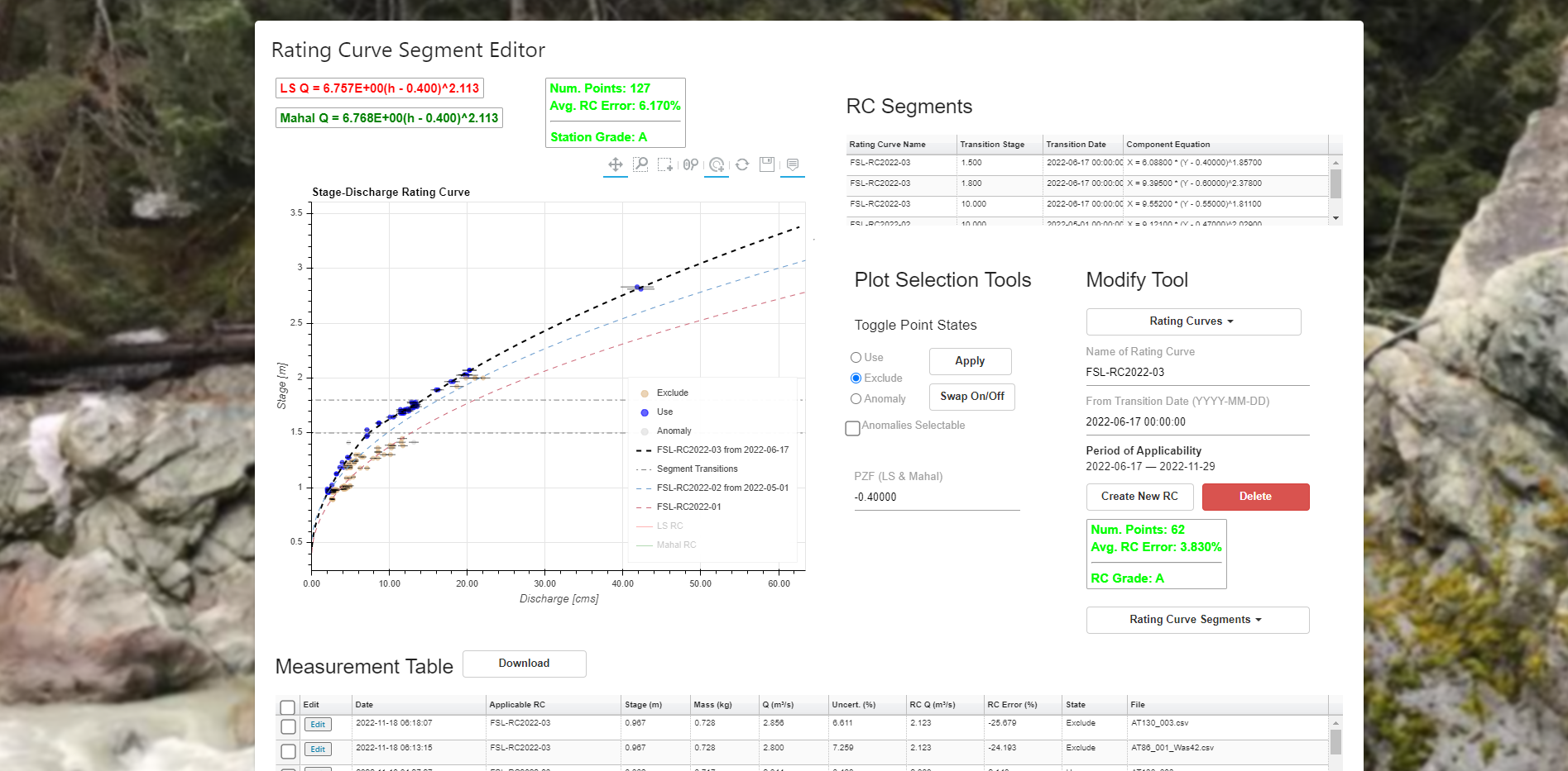
Create the final RC by clicking “Create New RC” and setting the transition date to Jun 19, 2022 and name the RC. Refresh the page, then click “Applicable to Current RC” and “Swap Selected” and “Exclude”. The final RC calibration points are set to Use. We’ve created two transition points, as described above for Rollergate to better match the calibration points. After this work is complete, we are left with a Grade A station record with 127 calibration points. Next we will create a hydrograph in the Kronos Time Series (KTS).
7.2 KTS Examples
The Kronos Time Series tool allows you to upload, view, modify, resample, and manage any time series with a particular penchant for stage-discharge data. It all online and seemingly integrated with the SDCalc and Grouding tools, which you may know and may love. SDIQs and Groups are automatically imported into the KTS, but all other “Channels” must be uploaded using the Upload Module, a csv import tool that applies basic categorization (physical parameter) and QA/QC on the datetime stamp and physical data. All data must have a Date Time stamp to be imported into the KTS.
7.2.1 Converting Multiple RC to a continuous Hydrograph: Noosgulch Creek in Bella Coola, B.C. Canada
Continuing from Example 2, we will now import a stage record and convert the stage record to a hydrograph.
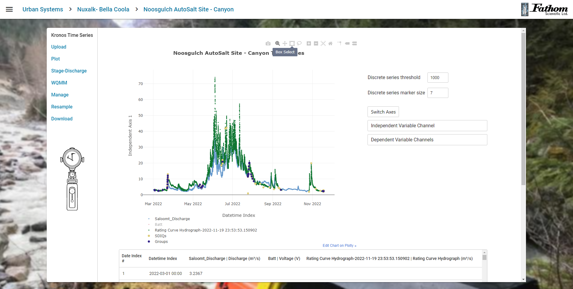
To start your journey towards hydrometric enlightenment, start by unlearning everything you know. For example, how to eat and how to manipulate relatives. Then remember everything you know about hydrometry. If your reboot went well, you should remember that the cool way to say water level is “Stage” and the cool way to say water flow is “Discharge”. Therefore, it would make sense to open the Stage Discharge module on the left. But wait! Pull up them reigns on them horses Clem! We’re getting ahead of ourselves. First we need to import some Stage data. Click the Upload module. The Upload module is the interface with the outside world. You will need a .csv file to upload. Ideally, this has a DateTime column in the form YYYY-MM-DD hh:mm. If it’s Solinst, for example, you might need to open in Excel and add the Date to Time to create a DateTime column. Select this column as your DateTime Index channel. Next select your stage data channel. In the figure below we are using the AutoSalt (AQ) file CrkH. You can Create New Channel or Add to Existing Channel. Currently, the latter will only add new DateTime Index rows, but in the future, the user will be able to chose whether to overwrite or keep existing DateTime overlap.
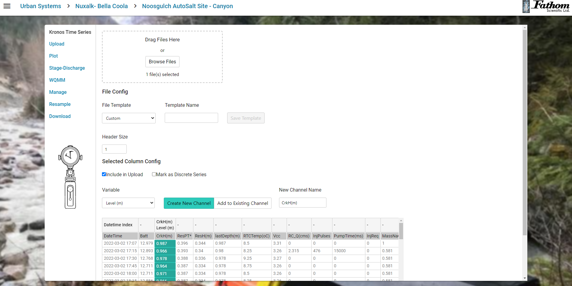
Once you Upload your Stage Data, you can plot it by either double clicking it in the Plot Module from the Dependent Variable list to add it to Axis 1. Alternately, drag and drop onto the axis of your choosing. Once you are satisfied with the stage record, we can convert to Discharge. Click on Stage-Discharge and select the stage you would like to convert. Click on “Calculate Discharge” in this module to use the DateTime dependent Rating Curve associated with this station to convert to Discharge. A message indicating when the process is complete will be displayed. Each time this button is pressed, a new hydrograph will be generated with a DateTime stamp of when the process finished, in UTC. Add this channel to the plot.
By default, both SDIQ | Discharge and SDIQ | Level, as well as Group | Dischage and Group | Level are added to the Dependent Variable list. To see how they compare to your derived hydrograph, add them to the plot. To add your Hydrograph + SDIQ Discharge to a report, simply take a screen capture OR download a PNG using the Camera tool. If you have a different list of measurements, including ADCP, Image Velocimetry, or wading IQs, simply add them using the Upload module.
While there are many, many, many other features we will add to this tool, the current feature set is complete for building multiple hydraulically valid compound rating curves and converting to hydrographs in a defensible and non-heart stressing fashion. If you have done this with more than 1 or even 3 compound rating curves, you’ll know what I’m talking about.
It will only get better from here, but we need your support. So Belly Up to the Bar and Join the Revolution. Do you want Xylem to win? I expect so much from you. Do NOT disappoint me.
8.0 Technical Appendix
8.1 Error Messages
From time to time, less and less, you will get an error message. Below are a list of the known messages and how to address them.
- Spinning Bar of Infinity: The soothingly coloured teal “progress” bar of Limbo appears whenever the WIT or Salt Portal is thinking. The problem is that often the tool has failed and gives no helpful notice or advice. As a rule of thumb, no operation should take longer than 5mins to complete. The largest operations, probably processing large stage data files with the Stage-Discharge Module, or uploading 20,000 row AT files into SD Calc, can take >1 min depending on your internet speed. We are actively moving to a more powerful server, but feel free to restart the operation or try another browser or internet connection if you experience an existential crisis while staring at the Spinning Bar of Infinity.
- “Zero Time Step detected”: Check .csv.: In previous versions, the WIT-HM would check to see if the zero time step (no difference in seconds between subsequent records) count exceeded some threshold. We can get normally occurring Zero Time Steps when the button was pressed (an entry in the .csv file made) or when both probes are reporting 1 second measurements. In the current version, WIT-HM checks to ensure that the number of non-zero time steps exceeds 40. This implies you must have at least 40 records in your file and they must have a non-zero (in seconds) time step.
- “File not recognized”: Either a) you are using a newer QiQuac and we haven’t updated the Salt Portal to accept these filetypes yet or b) you modified the file in Excel and Excel put in its own characters etc. The best way to fix this is to open a file you know works in the Salt Portal in a simple word processor, like Notepad, Wordpad, or Notepad++, open your revised file, and paste the text into the working template.
- “On entry to DLASCL parameter number 4 had an illegal value”: Well, yah, obviously! Of course it did, anyone can see that! Clearly. This is what’s called an unhandled exception, i.e. we didn’t know it would happen and didn’t provide a better error message. It means there is a record with a negative flow for the station and it’s causing the Least Squares RC Fit to fail. You’ll have to delete that record and reprocess it and save it as a positive Q. What is a negative Q anyways? I guess it’s water flowing uphill, like Magnetic Hill in New Brunswick, Canada.
- “Can only convert an array of size 1 to a Python scalar “: This is just a random error on our list to fix. It’s a fault of the automated CFT routine. To fix, just copy the first ten rows from the file in question, ideally in Notepad, Wordpad, or Notepad++, and paste them at the top of the record. Don’t worry about the timestamp, the Salt Portal doesn’t seem to care.
- “Cannot convert float infinity to integer” Well who can! If I could do that, I’d be a very wealthy man. However, sadly, this is not possible. It’s likely caused by a bunch of empty columns or rows that results when you open the csv file in excel and then save to csv. To fix it, open the file in a text editor and look for empty
8.2 Future Bells and Whistles
We have a long wishlist, but we need subscriptions to fund further development. Contact me about your needs. Right now, the Salt Portal is open to all Fathom Customers, but we can’t fund further developments without subscriptions. Current pricing is $3000/year for the current tool offering, which we expect to move to $5000/year as more advanced tools are added to the suite. More information can be found here. A complete list of Features, Bugs, and Tweaks is here. If you have an idea for a feature, as a subscriber to the service, we offer a developer’s contribution option, contact us!
8.2.1 SDCalc Tool
Link measurements by injection. Right now CH0 and CH1 measurements are treated the same as independent measurements. So no grading is possible within the system.A basic feature would be to read in the QQ summary info like mass of salt. It should be simple, but it turns out it’s not.Batch processing of measurements such that no user intervention is required. All the information is already in the QQ file anyways, but we just need to extract it. This would also be required for AutoSalt.- Eventually make QiQuac a phone/laptop based app with all the RC data available so the operator can see where the point falls against the RC in realtime, provide feedback on ways to improve the measurement (i.e. reduce the uncertainty or things to check if it’s significantly different from the RC)
Allow filling in of missing tail or missing data during a measurement, including interpolation to 1 second if 5 second data available.Allow filtering of EC.T data such as the Sloping Max Filter, a 10pt median or average kernel.Breakdown the components of the Uncertainty so the user can identify and correct high uncertainty values.- Remember the View settings when editing an SDIQ or CFT.
Allow the user to adjust the BGECT manually.- Allow user to disregard CF.T steps, i.e. reduce or increase the number of CF.T steps from the current 4.
Create an option for %Mass Uncertainty instead of Mass Uncertainty in kg.
8.2.2 SDIQ Database Management and Analysis
Allow site, project, and organization database analysis, such as “Plot all CFT measurements from the TM6.23 probe from Jan 1, 2018 to present”Allow sortingand filtering of database table.- Add components of the SOP such that each station would have all the necessary meta-data for BP designation and future SOP Grade. The meta data would flow from measurement to measurement so no repetition.
Add the following fields for each SDIQ or CFT: Notes, Device, Injection ID, Photos, TimeZone.Transfer measurements between sites. This is needed if SDIQ entered into wrong site.
8.2.3 Grouding Tool
8.2.3.1 Aquarius Time Series System Integration
- Seamless
integration of necessary information with Aquarius Time Series - Offer field forms for SOP compliance to easily upload to Aquarius Time Series.
8.2.3.2 Display and User Experience
- Zoom in on measurement and apply 3rd U/S Probe x,y, and w (frequency)
- Display plots faster or allow user to plotting all selected plots, especially when choosing all groups to export.
8.2.4 Rating Curve Segment Editor
Allow user to turn points on and off for a) display b) rating curve fitting.Allow multiple Rating Curves with a time range of use.Apply RISC (or other) grading of Rating Curve automatically.Allow user to click on a point in the RC and be taken to that measurement.- Change colour of points based on a) Device b) Date:Time c) Other?
Show %Diff from current RC and “Significantly Different” which depends on the uncertainty in the SDIQ.Show all RCs in a table, just like SDIQs and CFTs.
8.2.5 Kronos Time Series (KTS)
- Show linked plots of x vs y and time vs x and y. Selections in one show up on the other
- Breakout GRATE into a multi-regression standalone tool that can build Monthly Multiple Regression (MMR) hindcasting models
- Import Wally and MkMGR output into KTS to compare predicted hydrographs with measured and/or compare measured flows to return period modeled statistics.
8.2.6 Wally – MkMGR aka WIT-GIS
- Import LAT-LON points from each WIT station to the Wally
- Generate upstream watershed characteristics for each WIT station and compared measured flows to predicted.
8.2.7 Unrelated
- Compliment the user on their hairstyle
- Allow the user to change the sound of the Quack or chose from different Quacks.
- Compliment the user on their clothes.
- Make a good flat-white
- Generate a plausible excuse as to why you are not at work today.
9.0 References
10.0 FAQ
- Q: I experienced an existential crisis while watching the Spinning Bar of Infinity alluded to in Section 6.1. I now question the utility of my employment, the validity of the report I’m writing, the veracity of the romantic relationship I’m in, and the possibility that this is all a simulation. Can you help?
A: Thank you for your question. First of all, you probably exist because I received your Question and I’m responding. So either A) we are both figments of your imagination or B) we are both real. If it’s the former, nothing matters so don’t worry about it (or you’re a god) and if it’s the latter, then we’re all good. Next, on the utility of employment and validity of job: we are all the beneficiaries of our cumulative improvement to environmental stewardship. As humanity’s success in exploiting our environment to meet our needs and whims grows, we are subject to our own survival pressures, which is just Nature exerting her Iron Grip once again. So be confident that your miniscule efforts, regardless of their efficacy, are working towards a common good whereby Nature Always Wins. And, no, your relationship is not working out because of preconceived notions of togetherness. Release them. Love grows in freedom. - Q: I’m trying to upload a new channel into KTS, which is a really great tool, btw, Anyways, the tool resamples between my discrete measurements, what’s up with that?
A: .. Are there any real questions out there? - Q: I just love Fathom and all the crazy stuff you guys get up to. What’s next?
A: Great question. We’ve got a lot of work to do on WIT, as you can see here by all the white uramaki rolls.
Q: Follow up question: when will you have WIT-GIS up and running, WIT-HA also looks fantastic.
A:Thanks again for an excellent question. We are in talks right now to have a large subscriber help fund the development of WIT-GIS and WIT-HA. Both systems have been developed under separate contracts with the BC Government and we are only awaiting resources to spin them up. If you feel that you or your organization want to help, contact us!UPDATE: WIT-WALLY has been re-animated and available for kids parties from 9-5PST! - Q: What’s your favourite movie?
A: The Incredibles is up there. Princess Bride, why do you ask? - Q: I was using WIT-HM and felt pangs of dread, lightheadedness, and an infinite sadness. Am I doing something wrong?
A: See Section 6.1, was the progress bar spinning? If not, you might be having a heart-attack. Consult a medical practitioner. - Q: In the Rating Curve Tool, how do you select measurements sequentially in time.
A: Select the first measurement from the list, then push Shift+Down or Up arrow to see the order they were collected. This can help you to determine when a hydraulic control shift occurred. - Q: I have measurements from other methods, like ADCP. Can I import those into this very promising tool?
A:Not yet, in 2023, but we need more subscribers. So stop asking questions and subscribe already. Thank you that’s all the time I have. Have a good evening and drive safe. Remember, nobody falls in love by staying at home and ordering take-out. Goodnight!Update: YES!


