The following is adapted from “Introduction to Salt Dilution Gauging for Streamflow Measurement Part IV: The Mass Balance (or Dry Injection) Method” by Rob Hudson and John Fraser, with permission from the authors, published in Streamline Watershed Management Bulletin Vol. 9/No. 1 Fall 2005.  Italicized text is taken verbatim from the article, non-italicized text is by the author of this post and modified with [G.S.]

In part one of this series, Moore (2004a) introduced the general principles of stream gauging by salt dilution. In subsequent articles, Moore (2004b, 2005) described techniques of constant-rate injection and slug injection using salt in solution. This is the final article in the series and details the “mass balance method.” Originally described by Elder et al. (1990), the mass balance method differs from slug injection using salt in solution (Moore 2005) in that it is based on conservation of tracer mass, not of tracer volume. By using the mass balance method, salt can be injected into the stream either in dry form or in solution. Because it is more common to work with dry salt, this method has also become known as the “dry injection method.”
Dilution methods have been used for at least five decades (Østrem 1964; Church and Kellerhals 1970; Church 1975; Day 1976, 1977a, 1997b; Hongve 1987; Johnstone 1988; Kite 1993). In 1998 we began to develop the mass balance method for use in small BC streams where current metering is either difficult or impossible (Hudson and Fraser 2002). Subsequently, we have applied this method successfully in several coastal streams including Russell Creek (Hudson and Fraser 2002), upper Nahmint River on Vancouver Island, Flume Creek (Sunshine Coast), and Culliton and Furry Creeks (Sea-to-Sky Highway).

Background

The basic principle of dilution gauging is to add a known quantity of a tracer to a stream and observe its concentration in the stream at a point where it is fully mixed with the flow.  The higher the flow, the more it dilutes the tracer.  Dry salt used as the tracer must be injected at a point that favours rapid dissolution.  This creates a salt solution in situ that then disperses into the flow aided by turbulence in the water column.  The resulting concentration of salt is measured as electrical conductivity at a point downstream of the injection point where it is completely mixed.  The distance between the injection and measurement points is known as the mixing length (L).  The dispersion pattern of conductivity over time is similar in shape to a storm hydrograph (Figure 1).  Streamflow Q is calculated using equation 1 where M is the mass of salt (in grams) and A is the area under the graph of concentration over time (Figure 1).  The units of A are milligram-seconds per litre (equivalent to g · s/m³).  The quantity A in equation 1 and shown on the graph (Figure 1) can be calculated as:where c_t is the concentration of injected salt at time t, and t_int is the time interval between successive data points. As noted above, the salt concentration is measured as electrical conductivity (EC) in the stream. The concentration of the injected salt can be calculated using equation 3 below:where EC_t is the electrical conductivity at time t, EC₀ is the baseline conductivity, and CF is the concentration factor. The concentration factor is the coefficient in the near-linear relation between EC and salt concentration. However, CF is not a constant, since stream temperature and background chemistry also affect EC. These effects constitute a potential source of error that can only be controlled by understanding the relationships between EC and salt concentration, stream temperature, and chemistry. 

Salt Concentration

For a salt dilution measurement, both the background ion concentration in the stream and the concentration of salt added to the stream affect the CF. Hongve (1987) found that the concentration factor was directly related to the baseline conductivity of the stream. For a pure NaCl solution, 1 mg of NaCl added to 1 L of de-ionized water will increase conductivity by 2.14 μS/cm (CF = 0.467). As the ionic strength of the solution increases, the interaction of ions in solution begins to hinder each others’ activity. The CF is equal to 0.47 for [NaCl] in the range from 0 to 30 mg/L (EC from 0 to 64 μS/cm) and increases to 0.51 for [NaCl] in the range from 300 to 1000 mg/L (EC from 617 to 1990 μS/cm). However, the presence of ions other than NaCl in the stream being measured may result in a slightly different range of values for the CF. The relationship between EC and temperature is more-or-less linear in the range of temperatures commonly encountered during flow measurements, but there is considerable lack of agreement in the literature concerning that relationship at low temperatures (i.e., 0–3°C). Smart (1992) found a linear relation for temperatures ranging from less than 1 to 10°C, contradicting statements by Østrem (1964) and Collins (1978). Johnstone (1988) reported linear relations for temperatures from 0.5 to 25°C.

[G.S. Calibration Factor

There has been considerable research into the Derivation, Uncertainty, and Variance of the Calibration Factor used in Salt Dilution Flow Measurements since Hudson and Fraser (2005). This article discusses the results in more detail. The summary from that article are as follows:

1. 1. Use Temperature Compensated EC (aka EC.T), non-linear function (nlf) temperature compensation if possible, or 2.0%/˚C if not, compensated to 25 ˚C.  This recommendation promotes consistency across measurements, devices, and sites and reduces uncertainty due to temperature changes during measurement or CF.T.
   2. Calibrate your meters and record calibration.   Use CF.T to track calibration.
   3. Not all meters are appropriate.
   4. Our study suggests that CF.T is 0.486 ±2.8% at 95% confidence for samples tested.
   5. If using diluent in standard other than stream water, dilution correction should be applied.

This study suggests that insitu calibration (CF.T) may not be required for every measurement. Calibration to absolute reference standards in the lab, proper device settings (EC.T), user training, and appropriate corrections may result in LOWER error in derived Q and faster measurements in the field.]

Application of Dry Injection at a Stream-gauging Site

A stream-gauging site that is not suited to current metering or other methods (weir, flume, etc.) might be gauged by dry injection salt dilution. The following list outlines the criteria that should be considered before applying the method.

Preliminary criteria

Evaluate the site for suitability.  The basic characteristics of a reach suitable for salt dilution are:

1. Turbulent at all flows.
2. Steep gradient: Some channels with gradients between 3 and 5% can be measured with salt dilution.  Low gradient (<3%) reaches tend to be suitable for current metering and high gradient (>5%) for salt dilution.
3. Minimal pools and other backwater areas.
4. No tributary inflows in the gauging reach.
5. Riffle–pool, step–pool, cascade–pool morphology with cobble–boulder bed and flow constrictions.
   The above criteria are easy to evaluate at a field site.  However, the most critical considerations in applying the method are:
6.  Ability to perform a clean injection at a point that favours mixing and rapid dissolution.
7. The salt must be fully mixed with the flow at the point where EC is measured in the channel.

To meet criterion #6 is simply a matter of technique.  For “clean injection,” all the salt is injected into a point of turbulence with a single movement. [G.S. Subsequent research has shown that the time of injection is not important in the final estimate of discharge and that a slow injection over 30-60 seconds can ensure proper mixing and dissolution, and reduce the stress to aquatic species.]  The method may still work if the salt is injected in stages, but it will be difficult to determine from the dispersion graph if the measurement has been successful.  The ideal injection point is a constriction in the channel where most of the flow converges and passes between boulders in the channel bed.  For example, at Stephanie Creek a series of constrictions as the channel passes under the bridge (Figure 3) makes it an ideal injection site for two reasons:

1. the bridge can be used to dump the salt directly into the injection point; and
2. the turbulence created below the constriction helps to dissolve the salt and mix the resulting solution into the water column.

Criterion #7 is more difficult to verify because it cannot be determined directly without deploying numerous probes in the channel.  Choosing an appropriate mixing length is by far the most difficult aspect of the field procedure and requires an understanding of the dissolution and dispersion processes of salt in flowing water. 

Behaviour of injected salt in a stream channel

The dissolution of salt in water takes time, with the rate of dissolution being proportional to water temperature (i.e., it dissolves faster in warm than cold water) and inversely proportional to the existing concentration of salt.  This dissolution behaviour can be easily observed: salt dropped into a glass of cold water will dissolve slowly because the water surrounding the grains has a high concentration, and tends not to mix with the water above it.  However, once stirred the salt dissolves immediately.  The rate of dissolution is more sensitive to concentration than to temperature.  For dry injection at medium to high flows, the dissolution occurs at the lower concentrations.  As noted previously, dissolution is greatly enhanced by a good injection point such that even in glacier-fed streams where water temperatures are in the 1–3°C range, it can be assumed to occur instantaneously.  For low flows, and particularly in wide channels with limited turbulence, the salt can be dissolved in a bucket of water before injection to aid mixing.  This does not alter the method as long as the salt mass is known and fully dissolved in the water. 
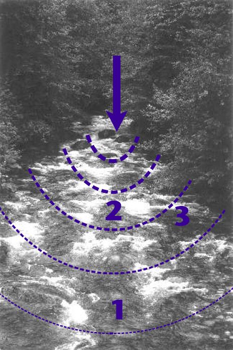
After injection, the salt mixes into the stream by longitudinal dispersion, a process in which dissolved salt in the plume moves along its concentration gradient until a uniform concentration exists.  The dispersion process is superimposed on the flow (hence the term “longitudinal”), which means that the plume extends downstream faster than it does towards the banks (Figure 4).  In this figure, the line that is farthest downstream represents a state where the salt plume approaches full mixing, making point 1 in Figure 4 the best location for the conductivity probe.  At any time during the measurement the salt concentration is higher at point 2 and lower at point 3 than it is at point 1.  Therefore, locating the probe at point 2 will yield a quantity A, which is too high, resulting in an under-estimate of the flow.  Similarly, if the probe is at point 3, A will be too low and the resulting flow estimate too high.
[G.S. A probe anywhere along the furthest downstream line, or further downstream, should yield the same result.  That is why it is recommended that two probes are used, either on each bank, or up and downstream, or mid-channel and bank, depending on the particular site characteristics.]

Calibrating the Site: Mixing Length and Dosing Ratio

A conservative guideline is that the mixing length should be about 20 times the average channel width (Hudson and Fraser 2002). While Day (1977b) recommends mixing lengths of 25 times width (25XW), this is probably a conservative estimate since channel width is usually estimated visually. In most cases this can be assumed to be a “safe” mixing length.  However, we have found that the optimum mixing length is often as low as 10 times the channel width, but users of the technique should conduct multiple trials to establish both the optimal injection points and mixing lengths for low and high flow at a particular site. 

Determine the optimum mixing length

Since the rate of dispersion of the salt plume depends on several factors, each site will have a characteristic optimum mixing length. To determine this length, collect a sequence of measurements by varying the mixing length under stable flow conditions.  The optimum mixing length is found where further increases in that length result in no relative change in the flow estimate.

Example of mixing length calibration

Culliton Creek is an ideal salt dilution site consisting of a long, straight reach with uniform gradient.  The morphology consists of a series of evenly spaced steps alternating with flow constrictions at each step.  At Culliton Creek two EC probes were used and two different injection points for 4 mixing lengths (Table 1; Figure 5). The channel is 10 m wide and the probes were deployed in mid-channel about 15 m apart. Two injection sites were chosen: the first site was about 70 m above the upper probe and the second about 30 m farther up the channel above the first injection site.  This resulted in 4 measurements at increasing mixing lengths (Table 1).

This procedure shows that the minimum mixing length at Culliton Creek is 100 m, or 10 times the channel width.  A standard methodology therefore in determining the optimum L might involve varying the mixing length from 10X to 20X the average width in 10- to 15-m increments. For high water, the relatively high flow velocity that typifies steep channels suggests that the mixing length should default to 20X the channel width.

Determine optimum salt dosing

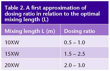
To apply dry injection for flow measurement, the injection mass must be known.  This requires an accurate scale and a means of packaging salt for use in the field.  Zip-lock freezer bags can easily hold up to 2 kg of salt.  Bulk salt (usually obtained in 20-kg bags from a bulk food distributor) can be pre-weighed into packages of various masses that can be made up in the field to the desired amount.  These bags can be carried to remote sites in a backpack.  Empty bags are weighed upon return to the lab or office to account for any residual salt not injected.  The final step to determine salt dosing for a new site is to adjust the dosing mass needed to get a clean signal.  In an earlier report (Hudson and Fraser 2002) we recommended dosing at the rate of 2 kg/m3/s of flow (dosing ratio = 2).  Since then, we have found that in many cases the dosing ratio can be as low as 0.5.  The aim of salt dosing is to add enough salt to get a clean signal without exceeding the most sensitive toxicity threshold (Moore 2004a, 2004b) of 400 mg/L NOEC (no observed effect concentration) for Rana breviceps (frog).  To get a strong signal, the difference between baseline and peak EC should be at least 100 times the resolution of the probe.  Optimum dosing ratio is related to the optimal mixing length;  the longer the mixing length, the more salt is needed.  At a mixing length of 10XW, a dosing ratio of 1.0 works well.  For longer mixing lengths, more salt is often needed for a clean EC signal (Table 2). [G.S. we have found similar results, but related the recommended dosing to sensor resolution (uncertainty) and transit time]

Limitations

Understanding the limits of applicability of dilution gauging methods in general will help to determine the appropriate technique for a given gauging site and whether to trust individual measurements.  Operators should document their observations, thus contributing to a systematic assessment of the limitations of any technique and leading to informed decisions about their choice.  Here are some of our observations regarding the limits of applicability of the mass balance method:

1. Instream conditions: Turbulence is all-important.  As a rule of thumb, conditions that violate the assumptions of current metering favour salt dilution and vice-versa.  When applying the mass balance method with dry salt, try to observe the salt as it is injected.  If it falls to the bottom of the channel and sits there in clumps, dry injection will not work. [G.S. it is possible to inject the salt either pre-dissolved or very slowly in cases like these. If the salt falls to the bottom, kick it to mix it up, the measurement should not be affected] Either dissolve the salt or use constant rate injection or current metering.  Some channel conditions render any method of measurement difficult or impossible. These include low flow conditions in very wide channels where the flow is dispersed by channel sediment.
2. There are situations where injected salt may be absorbed by (or may adsorb to) vegetation in the channel or other substances (e.g., neoprene chest waders).  Try to avoid applying salt dilution in channel reaches with a lot of aquatic vegetation. Always inject the salt in a downstream direction and, if possible, keep out of the channel during a measurement.
3. Violation of assumptions. In practice it is difficult not to violate some assumptions such as pools in the gauging reach. In riffle–pool channels, this is problematic since violation is a matter of degree — it can be minimized but seldom eliminated.  If pools are large relative to channel area, then the salt will hang in the pool resulting in an extended tail. In some cases, pooling results in less than 5% error due to cutting off the tail of the distribution (Hudson and Fraser 2002) but the error will be systematic (i.e., it will tend to give an over-estimate).
4. Examine the conductivity-over-time graph.  A clean dump with adequate dosing and full mixing has a characteristic shape.  Many common problems can be detected this way:
   1.  A smooth graph with a strong peak and short tail indicates a good chance of success.
   2. Irregularities in the graph could indicate low dosing, improper mixing, or other problems that could render a measurement unreliable. For example:
      1. Double peak — is it lack of mixing or is it discontinuous injection?
      2. Extended tail — does it indicate pooling of salt or a changing baseline?

This list of limitations is not comprehensive. The operator should recognize that documentation of observed limitations will lead to improved confidence in the application of dilution methods.  There is no substitute for experience in applying salt dilution gauging.  Over time an experienced operator will be able to judge the applicability of the method to a given site.

Comparison of Solution Injection and Mass Balance (Dry Injection) Methods

The mass balance method and slug injection of salt in solution method require similar calculations and both possess similar requirements for selecting a suitable measurement reach.  Both methods also require full lateral mixing of the salt in the stream and measurement of conductivity over time at a point downstream.  The mass balance method was developed for ease of application in the field.  Solution injection with saturated (20%) solution requires the operator to manipulate a slug that is approximately five times more massive than a dry salt slug.  In practice, a saturated solution is difficult to create in the field — a solution of 10–15% is more realistic.  Using 0.5 kg of salt per cubic metre per second as a guideline to assess the upper limit of applicability and if the flow is 10 m³/s, dry salt will require the operator to inject at least 5 kg of salt while solution injection will require about 35 L, or approximately 35 kg, of solution to be injected. While this amount may be manageable, the ratio makes dry salt injection more appealing at higher flows.  For example, we have measured flows greater than 40 m³/s with dry injection.  To use solution to measure the same flow would require at least 300 L of solution. Thus the practical upper limit of applicability of the salt dilution method by solution is in the range of 5–10 m³/s.  The use of dry salt instead of salt solution allows the upper limit to be extended to 100 m³/s or more.  
Another advantage of the mass balance method is that it requires less equipment than the solution injection method (Table 3).  The solution method requires the creation and calibration of injection solution for each measurement.  This requires more time on site and more equipment to be carried to the field as well as more opportunity for error in calibration.  Salt solution has an advantage over dry injection in that it will mix more readily in lower, less turbulent flow, since the salt is already dissolved in water. However, the mass balance method can also be used with solution as a known mass of salt can be dissolved in a bucket of streamwater before injection and the calculation carried out as though it were a dry mass.

Summary/Conclusions

Whether using solution or dry injection methods, the operator needs to have equipment for measurement and calibration.  As long as the application criteria are met, it makes little difference which method is used.  Both methods are capable of high precision.  We have tested the mass balance method with dry injection under a wide range of conditions.  Its speed and simplicity of application in the field make it an operational standard hydrometric method for small, steep streams.

Acknowledgements

We thank Dan Moore and others (anonymous) for their useful review comments. Thanks are also extended to Shelley Higman and Derek Ferguson for assistance with funding, Bill Walker (Water Survey of Canada) for current metering, and Dennis Morgan (Via Sat Data Systems) for testing methods. This work was funded in part by Forest Investment Account (FIA) and Forest Renewal BC, but primarily by the authors.  Any errors in this manuscript remain solely those of the authors. 

References

Church, M. 1975. Electrochemical and fluorometric tracer techniques for streamflow measurements. British Geomorphological Research Group. Technical Bulletin #12.
Church, M. and R. Kellerhals. 1970. Stream gauging techniques for remote areas using portable equipment. Department of Energy, Mines and Resources Canada, Ottawa, Ont., Technical Bulletin #25, pp. 55–68.
Collins, D.N. 1978. Hydrology of an alpine glacier as indicated by the geochemical composition of meltwater. Zeitschrift für Gletscherkunde und Glazialgeologie 13(1/2):219–238.
Day, T.J. 1976. On the precision of salt dilution gauging. Journal of Hydrology 31:293-306. Day, T.J. 1977a. Field procedures and evaluation of a slug dilution gauging method in mountain streams. Journal of Hydrology (NZ) 16(2):113–133.
Day, T.J. 1977b. Observed mixing lengths in mountain streams. Journal of Hydrology 35:125–136.
Elder, K., R. Kattelmann, and R. Ferguson. 1990. Refinements in dilution gauging for mountain streams. In Hydrology in Mountainous Regions. I – Hydrological Measurements; the Water Cycle. International Association for Hydrological Science Proceedings of two Lausanne symposia, August 1990. IAHS Publication No. 193, pp. 247–254.
Hongve, D. 1987. A revised procedure for discharge measurement by means of the salt dilution method. Hydrological Processes 1:267–270.
Hudson, R. and J. Fraser. 2002. Alternative methods of flow rating in small coastal streams. B.C. Ministry of Forests, Vancouver Forest Region, Nanaimo, BC. Extension Note EN-014 Hydrology. 11 p.
Johnstone, D.E. 1988. Some recent developments of constant-rate salt dilution gauging in rivers. Journal of Hydrology (NZ) 27:128–153.
Kite, G. 1993. Computerized streamflow measurement using slug injection. Hydrological Processes 7:227–233.
Moore, R.D. 2004a. Introduction to salt dilution gauging for streamflow measurement: Part 1. Streamline Watershed Management Bulletin 7(4):20–23.
Moore, R.D. 2004b. Introduction to salt dilution gauging for streamflow measurement Part II: Constant-rate injection. Streamline Watershed Management Bulletin 8(1):11–15.
Moore, R.D. 2005. Introduction to salt dilution gauging for streamflow measurement Part III: Slug injection using salt in solution. Streamline Watershed Management Bulletin 8(2):1–6.
Østrem, G. 1964. A method of measuring water discharge in turbulent streams. Geographical Bulletin 21:21–43. Smart, C.C. 1992. Temperature compensation of electrical conductivity in glacial meltwaters.