This article is based on material presented at the AWRA Conference in Virginia, USA, Nov 2014 (AWRA_Salt_Dilution_CFT_V0.3) which was co-authored by Gabe Sentlinger (ARD), Mark Richardson (UBC), Andre Zimmerman (NHC), and John Fraser (ARD)†.

Abstract

The Calibration Factor – Temperature Compensated (CF.T) is the relationship between NaCl concentration ( [NaCl] ) and conductivity.  The CF.T is required to convert the conductivity-time signal in a Salt Dilution flow measurement to [NaCl]-time.  The relationship is nearly linear (R² = 1.000) over the range of interest (~100 μS/cm).  There appears to be some chemical interaction at higher concentrations which changes the CF.T slightly.  In our study, we have not found that the CF.T is not significantly affected by a range background chemistries, nor Background Electrical Conductivity (EC_^BG).  We have also found that measuring CF.T is non-trivial and many considerations must be made.  This post describes the study conducted and the preliminary results.

Introduction

One of the original motivations behind this study was autonomous salt dilution gauging (as demonstrated in Figure 1).  Fathom has developed the AutoSalt system for unattended flow measurements.  However, no in situ derivation of the CF.T is performed.  In our experience, the CF.T does not vary significantly.  The questions we were faced with was:

• How much error is introduced by assuming a CF.T for automated measurements?
• Is CF.T a function of BG EC.T or chemical makeup?
• Is CF.T a function of the instrument (it shouldn’t be, since it has physical units)?
• Does CF.T vary by region (chemical makeup)?

These same questions pertain to manual measurements as well.
Hudson (2005) states:

Hongve (1987) found that the concentration factor was directly related to the baseline conductivity of the stream. For a pure NaCl solution, 1 mg of NaCl added to 1 L of de-ionized water will increase conductivity by 2.14 μS/cm (CF = 0.467).  As the ionic strength of the solution increases, the interaction of ions in solution begins to hinder each others’ activity.  The CF is equal to 0.47 for [NaCl] in the range from 0 to 30 mg/L (EC from 0 to 64 μS/cm) and increases to 0.51 for [NaCl] in the range from 300 to 1000 mg/L (EC from 617 to 1990 μS/cm).  However, the presence of ions other than NaCl in the stream being measured may result in a slightly different range of values for the CF.

We have since challenged this finding and assumption.  Our investigations have found a strong bias is introduced if the CF.T is calculated using a standard solution made of dry salt and distilled water.  It was originally thought that using distilled water as a solute had no impact but to increase the volume of water in the resulting solution.  However, since that time we’ve found that when the solute has a concentration of salt that differs from the solution being tested, the effect is to increase or decrease the conductivity.  We believe that Hongve used a distilled water-based standard but did not correct for the addition of the distilled water.   We’ve derived two means to apply the “Distilled Water Correction”.

Distilled Water Correction

If using a standard solution for CF.T calibration, we need to account for the conductivity depression resulting from preparing the calibration solution with distilled water.  The depression is greater the higher the background conductivity of the stream water.  The predicted depression in electrical conductivity by adding a known volume of distilled water can be derived from a two-component mixing model:
(1)
Where EC.T_i is the Stream water EC.T, EC.T_dw is Distilled water EC.T, EC.T_mix is Mixed water EC.T, V_i is the initial volume of stream water, V_dw is the volume of distilled water added.  The resulting depression of conductivity (ΔEC.T) can be estimated by rearranging the above terms.
(2)
The ΔEC should be added back onto the EC.T_i to determine the correct slope (CF.T).   The CF.T was conventionally calculated using:
(3)
where EC.T’ was the resulting EC.T after adding V_dw to V_i.  CF.T_ms>> is the CF.T that resulted from the slope of the regression line between the EC.T and the change in [NaCl] if the mass of salt (m_s) was assumed to be very large compared to the salt introduced from the distilled water and that already in the stream sample.  To achieve EC.T_true, you should substitute EC.T’ with (EC.T’+ΔEC ).
(4)
To calculate EC.T_true in this manner requires reprocessing the calibration data for each measurement.
If the user would like to re-correct historical calibrations from summary data only, we’ve developed an analytical solution for that purpose.  The details of the proof are available upon request from the author, but the resulting correction is as follows:
(5)
where EC.T_d is the conductivity of the distilled water or diluent, EC.T_o is the conductivity of the original stream sample, and [s] is the concentration of the standard being added.  From this equation, we can see the correction is very small if either a) the difference between the EC.T_d and EC.T_o is small (i.e. stream water is used as the diluent) or b) the [s] is very large.  We do not mean to suggest that stream water necessarily be used as the diluent; we have found that this correction, or eq 4, results in a CF.T that is not significantly different from a CF.T derived using stream water as a diluent.  Conversely, the correction is large if EC.T_d is much smaller than EC.T_o, for example if a distilled water standard is injected into highly conductive late summer inland flow originating from groundwater sources.
In equation 5, CF.T_true is a variation of eq 4 given by:
(6)
where m_o is the mass of salt in the original sample, m_s is the mass of salt added to the std injection, m_d is the mass of salt in the distilled water or diluent.  In this version of CF.T_{true ,} we do not correct the EC.T for the distilled water (or whichever diluent is used), but we keep account of all the salts (ionic conductors) in the resulting solution.

Figure 2 shows and example of the original CF.T calculated for a very conductive sample.  In this example, ECi was 1142 uS/cm. Distilled Water EC.T was 2.2 uS/cm. This resulted in a depression of ~27% for each injection.   If the uncorrected EC.T was used, it would result in a 27% underestimation of Q. This CF.T can be corrected for by correcting each injection by ECmix and then recalculating slope (as shown in Figure 2).  This method requires reprocessing old calibrations. The CF.T can also be corrected for using the analytical approximation (-27.4% in eq 6).
(6)
Regardless of the method used to achieve CF.T _true, eq 4 or eq 5 (they agree within 1%), one of them should be used to avoid error if a prepared standard is used in the calibration.

Temperature Compensation

Before moving on to the expected variance in CF.T, it’s important to understand temperature compensation.  It is a neat quality of ionic conductivity by NaCl that the response to temperature is nearly linear.  The warmer a liquid is, the higher the conductivity.  Different methods exist for compensation.  As show in Figure 3, the best results are obtained using Non Linear Function (nlf) compensation (EU 27888).  The corrected EC. T values in Figure 3 show less deviation from a constant EC, especially below 10ºC.  However, nlf is not an option on all meters. The next best correction is linear 2.0%/˚C for NaCl.

Note that the departure of the linearly compensated EC from nlf compensated EC is not an issue for SDIQ if temperature is held relatively constant for CF.T derivation and over the course of the measurement.  However, this is not often the case, or difficult to obtain (i.e. glacier melt at near zero degrees and calibration done in warm summer weather).
Using EC.T and and CF.T, is best way to address temperature affect.  Also, using temperature compensations adds a layer of QA/QC to ensure linear and repeatable EC.T responses.
There may a possibility to reduce the time required for an SDIQ measurement if the operator can assume a CF.T, and permit accurate Automated Gauging.  However, even if we can assume a CF.T for a site, it is still necessary to ensure that all equipment is working properly and is properly calibrated.  The latter concern is reason enough to perform a CF.T calibration, but this study suggests that we can expect a CF.T value with a relatively tight variance.

Theoretical CF.T

Different Salts in solution have different slopes of EC.T vs [salt], which also change with concentration of the salt.  Figure 4 is again taken from Moore 2008 which is based on Molar Conductivities first presented in Harned and Owen (1958).   SD IQs should only increase the concentration by 10-20 mg/L, so the relationship remains approximately linear over that span of interest.
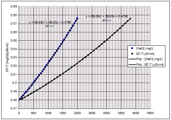
Figure 5 shows the theoretical EC.T vs. [NaCl] (taken from Harned and Owen (1958)).  It is not quite linear, but the polynomial can be used to estimate the [NaCl] from the EC.T at 25ºC, or vice-versa. The slope of the line in Figure 5 on the left at discrete values of [NaCl] can also be worked out, as it is in Figure 5 on the right.  We can see the CF.T increases with an increase in [NaCl].  The EC.T is also plotted so long as the increase in EC.T is only associated with an increase in [NaCl].  If another salt is present in significant quantity then the change in slope will not correspond to these EC.T values.  For most streams and rivers that we have worked in, the background EC.T is less than 500 μS/cm, often less than 100 μS/cm, so the expected CF.T value is ~0.485 (mg/l)/(μS/cm).

In order to test the accuracy of the theoretical CF.T values, several experiments were performed where a NaCl standard was added to a water sample and the EC.T measured and the CF.T derived.  The results are shown in Figure 6 and compares the experimental results to the theoretical CF.T relationship.  The first test was performed by M. Richardson using the same techniques and equipment employed throughout this analysis.  The 2-pt slopes are shown by points while the 5pt slopes by lines.  This requires that the series are offset from the EC.T of the first injection.  The EC associated with the 2^nd and 3^rd point of the slope calculations are shown. This test resulted in line slightly above the Harned & Owen line, but showing a similar trend with similar (+0.05) starting and ending points.   ARD conducted another series of experiments using our own lab equipment and a recently calibrated WTW330i handheld conductivity meter.  The goal was to compare our results to M.Richardson’s.  Our first set of tests were between 20-500uS/cm with smaller injection increments.  The results were interesting, shown by the dim solid lines in Figure 6, but highlighted an artifact of the equipment.  The WTW 330i autoranges at 200 uS/cm.  The resolution between 20-200 uS/cm is 0.1 uS/cm while it is 1 uS/cm above 200 uS/cm.  This jump to a coarser resolution was readily apparent in the 2 point slopes, and the 4 pt slopes showed an unexpected “step” in the CF.T values around 200 uS/cm.  Usually EC meters will change sampling voltages and frequency when changing ranges, and probably two separate calibrations are used.  Therefore it was not informative for the purpose of this study to sample with such fine resolution around the meter’s range boundary.
The next set of tests used large injection increments and ranged between 20-2000uS/cm. While the 2-pt slopes in this experiment show much more noise than M.Richardson’s, the 11 pt slope series show an uncanny resemblance to his 5 pt slope series, albeit offset by -0.07.  Both series were extrapolated back to zero using the lowest 5 points in the series.  These trend lines flank the theoretical Harned & Owen series at zero.  Both series exceed the Harned & Owen line between 200 and 1500 uS/cm, quickly climbing to >0.50 (mg/l)/(uS/cm) above 500 uS/cm.
This test confirms the dependence of CF.T on [NaCl], but also confirms that the CF.T can be assumed to be 0.485±0.01 (mg/l)/(uS/cm) in most streams where Salt Dilution is performed (0-200 uS/cm).

Variance of CF.T

We’ve undertaken a large sampling and analysis program of derived CF.T values throughout the Province of British Columbia.   This began as an internal exercise between nhc (A.Zimmerman) and ARD (G.Sentlinger) to quantify the variance of the CF.T value within our own records.  The results of this preliminary analysis is shown in Figure 7.  The nhc histogram on the left shows approximately the same distribution as the ARD histogram, however there are few differences.  NHC has plotted their histogram based on actual CF.T while ARD plotted theirs based on %Median of Site.  The latter shows only 5% variance at the 95% confidence interval.  This implies that if the user simply uses the median CF.T from historical calibrations, 5% uncertainty would be added into the resulting SDIQ.  Keep in mind that the calibration procedure itself adds between 2-3%, as discussed later in this article.
This finding may not imply that one need not calibrate at site, but rather the operator should expect to obtain a CF.T that is within 5% of the expected value.  If the operator calculates a CF.T that is significantly different than this value, it should motivate them to redo the calibration, check their equipment or procedure, or throw the calibration value out.
Also bear in mind that the slope depends on the kind of temperature compensation applied.  For NaCl, 2.0%/ºC is most accurate if NLF is not available, but NLF is most accurate below 10ºC.  The operator should ensure their meter is compensating to 25ºC.

The second round of CF.T variance analysis was with the help of Mark Richardson and R. Dan Moore from UBC.  Under the guidance of A. Zimmerman, hundreds of samples were analyzed in a lab setting and the results were encouraging.  Figure 8 shows two plots.  The figure on the left categorizes the CF.T by instrument.  From this figure we can see that both the WTW and CS547 shows the smallest variance and both agree with the theoretical value of CF.T.  The figure on the right categorizes further to separate out those CF.T values collected by M.Richardson to the highest quality control measures with a single instrument.  That category is “One User and one WTW many different creeks (n=40)”.  This impressive dataset has an average CF.T of 0.483 (mg/l)/(μS/cm) and a very tight uncertainty of only 1.6% at the 95% confidence interval.
 

This finding has several important implications:

1. with a quality instrument that is properly calibrated, it may not be necessary to perform an in situ calibration at each site, and only introduce 1.6% uncertainty into the derived SDIQ.  Remember that propagating the uncertainty through a  manual calibration introduces between 1.4% – 2.3%.
2. the CF.T is not a function of EC.T, as suggested by Hongve (1987) and Szeftel (2011).

Many of these tests were performed in a lab on samples taken from site several days prior, and cooled down to site temperatures.  This is an important finding.

Variance by Region

With the assistance of D.Hutchinson from WSC, we were able to perform CF.T calibrations on 40 samples from BC and Alaska with BG EC.T spanning from 3.9 µS/cm to 1142 µS/cm.  These points are shown in Figure 9.  Note that the x axis in this plot is logarithmic and the larger BG EC.T values have a CF.T of 0.48.  The most reliable measurements (from M.Richardson) are the series “A second WTW, one user”, which include the largest BG EC.T values.  There is no significant correlation between BG EC.T and CF.T.
This is an important finding.  Remember from Figure 6 that when the salt is NaCl added incrementally, the CF.T does increase to around 0.52 at 1000 µS/cm.  This implies that the ions interact with each other, impeding conductivity, only when it’s the same species.  No assay has been done yet on the 1142 µS/cm samples, but it is likely not NaCl which is causing such a large BG EC.T.

Figure 10 shows a map of BC showing location samples, BG EC.T and the CF.T.  There does not appear to be any spatial correlation with CF.T.  Inland samples tend to have higher BG EC.T.  Higher BG EC.T sites in Yukon yield larger CF.T, but only by 1% from the average.

Summary

There are many important findings in this study so far:

1. Use Temperature Compensated EC (EC.T), non-linear function (nlf) temperature compensation if possible, or 2.0%/˚C if not, compensated to 25 ˚C.  This recommendation promotes consistency across measurements, devices, and sites. and reduces uncertainty due to temperature changes during measurement or CF.T.
2. Calibrate your meters and record calibration.   Use CF.T to track calibration.
3. Not all meters are appropriate.
4. Our study suggests that CF.T is 0.485 ±1.6% at 95% confidence for samples tested.
5. If using diluent in standard other than stream water, correction should be applied.

This study suggests that in situ calibration (CF.T) may not be required for every measurement.  Calibration to absolute reference standards in the lab, proper device settings (EC.T), user training, and appropriate corrections may result in LOWER error in derived Q and faster measurements in the field.  We might not ready to do away with in situ calibrations as it ensures all equipment is working properly, but this study informs us that we should expect a CF.T around 0.485 +/-0.01 if everything is working properly.  It’s still possible to get a high quality measurement if your instrument does not produce this result, so long as the operator knows why it doesn’t result in a CF.T of ~0.485.

Acknowledgements

This study was made possible by the tireless work of Mark Richardson in support of his thesis at U.B.C. under the guidance of R.Dan Moore and Andre Zimmerman from NHC, and partially funded by the Mitacs program.  We also gratefully acknowledge the contribution from WSC for the water samples and logisitics, under the guidance of Dave Hutchinson.  A big shout-out to Jane Bachman from EDI-Whitehorse for providing high BG EC.T water samples to inform the upper end our data cloud.  Thank you to Robin Pike of BC MOE for providing helpful comment on the draft version of this study.

References

S. Harned and B. B. Owen (1958) Physical Chemistry of Electrolytic Solutions, 3rd edn, Appendix A, 697, Reinhold, New York.
Moore, R.D. G.Richards, (2008) and A. Story “Electrical Conductivity as an Indicator of Water Chemistry and Hydrologic Process” Streamline Watershed Management Bulletin Vol. 11/No. 2 Spring 2008 29, Victoria, B.C.
Moore, R.D. (2005) “Slug Injection Using Salt in Solution” Streamline Watershed Management Bulletin Vol. 8/No. 2 Spring 2005, Victoria, B.C.
†NHC: Northwest Hydraulic Consultants ARD: Aquarius Research & Development Inc UBC: University of British Columbia.