


Wally is the online implementation of a sophisticated GIS and Geo-Spatial Regression model coupled to Regional WSC hydrometric records to generate catchment GIS characteristics, and estimates of hydrological statistics. You can find a manual written by Paul Saso here. Below you will find alternate and supplementary background.
Instruction Manual for WIT-Wally
1.0 Introductions
Wally was a government of British Columbia project in 2021 to bring hydrological Prediction in Ungauged Basins (PUB) to the People. Fathom Scientific was tracked down in a travelling carnival near Prague telling fortunes and hired to develop the hydrological models intended for Wally’s brain. Hanging up his oracle’s robes, Fathom got to work spinning up the next iteration of the previously developed Modified k-fold Multivariate GeoSpatial Regression (MkMGR) models. These models use publicly available Geo-Stats (Slope, %Glacier, PRISM PPT, %Solar Exposure, Median Elevation, Drainage Area, PET) to predict common Hydro-Stats (Mean Annual unit-Runoff (MAR), Mean Monthly Discharge (MMD), 30Q5, Summer-7Q10, etc) based on a k-fold[1]approach. In this method well suited to small datasets, we train a multivariate regression model with a randomly selected sample of the dataset (usually QA/QC’d WSC flow data) for a particular Hydrological Zone (HZ) based on HZs defined in Obedkoff & Coulson (1998). A HZ is defined as..
an area with homogenous runoff characteristics where data can be reasonably extrapolated to estimate the characteristics at ungauged sites with an acceptable degree of accuracy. A hydrologic zone is typically identified based on physiographic features and/or a statistical study of hydrologic data. Due to the scarcity of hydrologic data in an extremely heterogeneous province such as British Columbia, this project used a physical mapping approach to delineate the hydrologic zones.
from “British Columbia Regional Streamflow Inventory Reports” accessed Dec 18, 2024
The “Obedkoff” reports originally published in 1998-2001 are invaluable resources for any BC-based hydrologist and provide the basis of the MkMGR approach. Where Obedkoff used median elevation or Drainage Area to predict common Hydro-Stats, we have used the same approach but expanded out the predictor variables to the seven geo-stats listed above. The updated reports by Ashfaque Ahmed are freely available on the Province of British Columbia website. Ahmed has also provided access to a very powerful webbased portal.
While we do not use the data presented in those reports, we use similar QA/QC procedure to select which data to include in the training sets. To derive the study hydro-stats, we use the R-Library FASSTR (Goetz et al 2024) run on the most recent version of Hydat. The key filters we’ve employed to retain the largest possible dataset and minimal short term effects are:
- >10 complete years of daily data AND
- A Wally DA within 20% of the Hydat DA AND
- <200%MAD Gross Allocation OR Net Allocation = Zero,
For a full discussion of these filters, along with the filters used by Ahmed, WSC (Hutchinson 2020), and a discussion of Naturalization, please see Sentlinger (2023). Regarding 2. If the DA calculated within Wally is outside of +/-20% of that calculated for the WSC station in Hydat, the training algorithm assumes of them is wrong and omits this WSC station in the training data. This approach strikes a balance between dataset size, recent climate change trends, and minimal regulation, with no controversial attempt to naturalize flows.
Wally is currently hard at work writing his story for publication as a white paper that can be referenced. Wally insisted the methodology be transparent, defensible, and repeatable, unlike his competitors. Until that time, we proudly present this abridged version with a short introduction to the tools.
Read more about Walter MkMGR’s Origin Story here, here, and ..over here.
1.1 General Overview
Wally’s Waking Hours are from 07:30 to 17:00 Monday to Friday (until the subscription base increases, you…)
Visit him here: wally.fathomscientific.com
Take Wally for a walk around the province! He can handle cross-border catchments, he can warn you about karst (Gahhhhh! he will say), he can generate very accurate watershed catchments for download (.shp) and predict various streamflow statistics with uncertainty bounds. He can measure and report catchment geo-spatial statistics, along with estimated licensed water allocations. He can generate an EFN analysis based on Water Sustainability Act guidelines. He can generate long-term hydrostats for WSC stations. He has many other talents and skills that have barely been tested (no exaggeration!).
1.2 Disclaimer
The Wally tool employs hydrological models that have not been peer reviewed. You can review previous studies here, here, and ..over here. We are asking for Beta Testers to assess the accuracy of the predictions. If you’d like to take Wally for a Walk, please contact us at info@fathomscientific.com, or just go ahead and report back.
1.3 Assess Water Availability
The main tool that has been developed is the Analysis > Surface Water Availability tool. To use it, first find your study catchment. This can be done using many different search function in the upper right of the Wally tool: place name, station name, coordinates, street address, etc. The Wally tool will take you to the location. To start an analysis, select “Analysis” and “Surface water availability”. The pointer will become a hand. Click near to a delineated streamline in the map and the tool will begin its calculations.

After a few minutes, the tool will report back the watershed modeling results, along with a shaded blue catchment in the map window. You can download this catchment as a shp file from the “Export” box above the watershed results table on the left half of the page. You can also download an excel version of the watershed results.
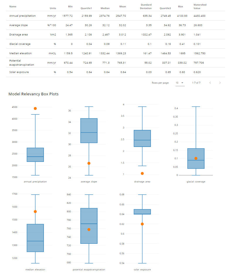
Another useful output is the geo-spatial stats from the catchment, shown below. Wally calculates the 7 catchment parameters used for the regression analysis. Additionally, Wally reports the HZ. The HZ is from the point of interest. If the user knows that the center of the catchment exists in a different HZ, they can enter the other HZ into this field. Indeed, it is possible for the user to enter any value into these boxes and re-run the model by clicking “Apply”, shown in Figure 1.3.2
It’s important to note that most of the MkMGR models are normalized by Mean Annual Discharge (MAD). That means that to train the models, we divided all the hydro-stats first by MAD, and then trained the model. To get the model results, for S-7Q10 for example, it’s necessary to multiply by model results by MAD for this study site. This results in more accurate estimates of the hydrostat, relative to MAD, but means that that the total uncertainty is the sum of the %Hydro-Stat Uncertainty + the %Uncertainty for MAD. This allows the user to enter in a known MAD if they wish to know the S-7Q10 for their site to improve the estimate. Also note that the estimate of MAD is also normalized by Drainage Area. We model the Mean Annual unit-area Runoff in l/s/km² and measure the Drainage Area. Yes, we are working on a paper for the method and the tool.

There are many tools and features in the Wally, including a provincially developed EFN model comparing licensed use to estimated water availability, shown in Figure 1.3.3. In this example, the licensed allocation is for a run-of-river hydropower project.

Because the model is stochastic in nature, it is possible to estimate the uncertainty on every geo-stat. These are included in model output, under Model Calculations and Error, shown in Figure 1.3.4

In addition to the uncertainty analysis, Wally is hard at work showing where within the training data your study catchment resides. For example, Tyson Creek shown above has a median elevation of 1563mASL, where the training data ranged from from 1159 mASL to 1695 mASL in this HZ. The whisker-box plot shows that it is in the training range, unlike the PPT and the DA. When study site values are outside +/-15% of the training range, the value input to the model is throttled to +/-15% of the range, and the user is warned. For example, in the case of Tyson Creek, the drainage area of 10.98 km² (10^1.04) is throttled to the lowest value in the training set (10^1.365)*0.85 = 10^1.16. The Drainage Area of 1.98 km² is still used to multiply the Mean Annual Runoff (MAR) by to get Mean Annual Discharge (MAD), but the HydroStat models that use DA as a predictor variable in the Multiple Regression uses 10^1.16 instead of 10^1.04. This throttling was determined analytically to minimize extrapolation errors (Sentlinger, 2017b).
[1] The k-fold approach may have been developed as early as 1931 (Larson 1931) but the exact origin is unclear (Wikipedia 2024). We developed the modified k-fold approach independently.
1.4 Wally’s Other Facets
Wally is anything but simple. In fact, he’s quite multi-faceted and complex, as he likes to brag/moan at the dinner parties he’s rarely invited to. Wally was intended by the BC Government to be a multi-purpose water use and availability tool, hence there are multiple tools that the author has no idea how they work. For example, the Cross-Sectional Well tool will find all the wells within some distance of a polyline or polygon that the user draws.
Please refer to the embedded documentation for hints on how to use Wally’s other facets. We’ll continue to develop this manual as time goes on and we learn how to use the tool we host (lol).
1.4.1 Groundwater Analysis Tools
The two groundwater analysis tools, found under the “Analysis” tab, provide users with excellent information and visualizations about existing groundwater wells, as well as the potential interaction between wells and surface water.
The Cross Section Plot, shown below, allows users to quickly see how wells along a chosen path relate to each other in terms of depth, water level (as measured at time of construction), as well presenting Aquifer Lithology and material where available. All the wells shown are linked to the provincial database allowing quick access to more detailed information about each well. The visualization mode can be set to 2 or 3D modes depending on user preference.
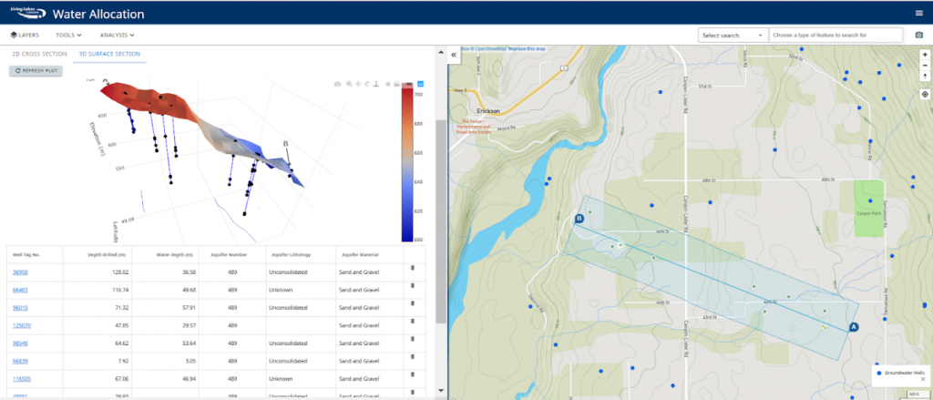
Figure 7 – Groundwater Cross section plot
The Hydraulic Connectivity Analysis (Figure 8) presents users with a starting point for evaluating interactions between a selected groundwater point and the surrounding streams. The tool calculates the distance to the ten nearest stream segments from the user selected point. It then identifies the closest point on each stream segment and uses the distance from these points to compute what the apportionment value is based on an inverse distance method.
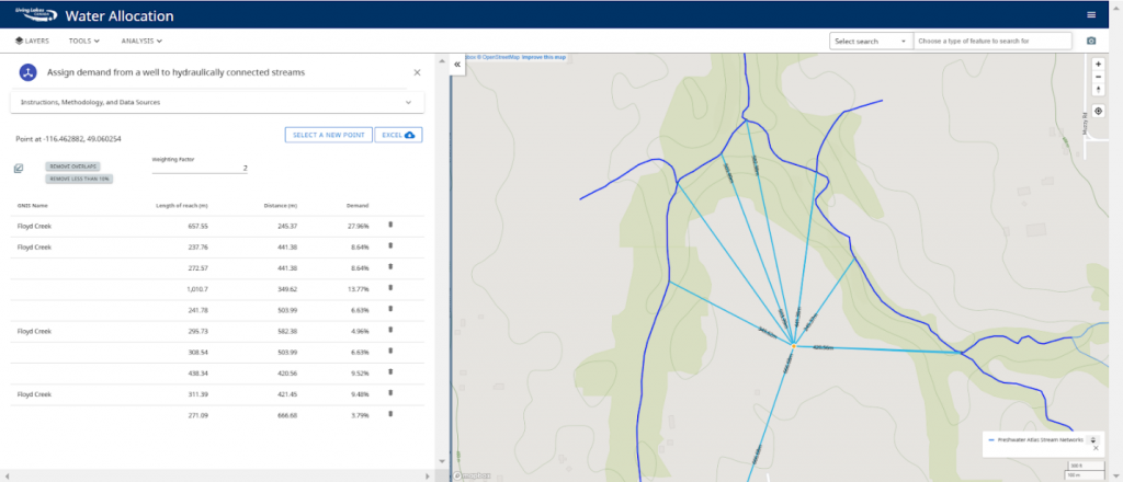
Figure 1.4.1 – Hydraulic Connectivity Analysis
1.4.2 General Tools and Layers
Under the “Tools” menu, users can select to search for water licenses or groundwater wells by selecting a point of interest or drawing a polygon around an area of interest. Users can also calculate distance and area on the map interface.
By clicking on the “Layers” tab users can select from a wide variety of geographic information to display in the map window.
2.0 Walter MkMGR’s Origin Story: An Optional Fathomland Tall-Tale
Walter MkMGR started out as a sweet Scottish Highland lad, on the sunny shores of Nairnia, just west of Westerberg. He often found himself in trouble with the law due to his proclivity for monkeyshines. Upon graduation from Fathom Highlands High in 1912, with honours in machining, he signed up with the Black Watch (the Fathom Highland Fuseliers) as a submarine mechanic, and volunteered for active duty against the little known Threat of Morsem Nuclear subs in the Black Sea. Wally proved his mettle during a freak nuclear meltdown, caused when somebody’s (nobody claimed responsibility) grilled cheese sandwich, which was grilling on a nuclear core, slipped between two plutonium rods and caused them to overheat. Wally (who just happened to be nearby) sounded the alarm and attempted to retrieve the grilled cheese sandwich while his fellow seamen escaped. The story goes that he did retrieve the sandwiched sandwich, but was badly poisoned by radioactivity in the process (there was also tell of a large bite out of the grilled cheese). His seaman friends found him unconscious, with crumbs on his mouth, in the nuclear core, and stark naked (no explanation given). After a lengthy convalescence (where he met, wooed, and fell in love with his nurse Esmerelda LeCove) he was startled one day to find a lump growing from both his armpits. “Swollen lymph nodes,” said the doctors skeptically. But the lumps grew and before long, Wally had sprouted 2 additional arms.
Shun from traditional society, and eschewed by Esmerelda, he moved north. There he wandered the hills, and learned the lay of the land, the movement of the water across the land, and the affect of the slope, elevation, drainage area and solar exposure on the timing and volume of runoff. He met an old man in the mountain hills, Murray, Old Man Murray, who taught him to play the bagpipes and together they fashioned a set for Wally. Old Man Murray had been confined to his cave in the Carleton mountains for decades, where he studied the advanced topics of Potential EvapoTranspiration (PET) Precipitation (PPT), and Glaciers (GLC). While his initial attempts at playing were met with more scorn and even further shunning, like most bagpipers he continued on, loudly, resolutely, paying no attention to social cues until the locals expected to hearhis shrieking melodies each morning. The particular tune would foretell of floods and droughts, 10% Percentile flows and Summer- 7day average 10 year return monthly flows. Together Wally and Murray roamed the highlands giving council to local hamlets, townships, and even on occasion the grand metropolis of Meganopolis.

With the tales of their prophecies in ungauged basins traveling far and wide, King Nick of Everard caught wind of his abilities. King Nick had spent several years perfecting a beast to predict flows, incorporating the Dark Magik of his Sorcerer Zorkin. The Magic was known only as XGBoost and Archmage Zorkin created a beast, half shark, half automon, and embued it with the power of XGBoost. King Nick wished to be entertained and to entertain his subjects. In the Christmastime of 1921, he invited various mages from around Fathomland to face his beast in the arena of hydrological prediction. The beast was enormous, measuring 17′ in height and almost as wide, in girth, but only 15′, so… pretty close.
XGBoost destroyed the other champions, tearing them limb from limb with obscure terms like “gain” and “coverage”. The black neural net would shoot out on the competitors and blind them to reason until they squirmed in a mealy mess of near perfect predictions. The glass dome would retract painfully slowly and then… consumption. MkMGR likewise wasted through his competition with his added appendages and striking cacophony, competitors like the slipper NEWT fell by his wayside. The carnage continued until only two remained: Walter MkMGR the young upstart from the Highlands, and XGBoost, the mechanized monster of methodic mayhem.
The final match was planned for Christmas Day,

All the Fathomlanders had gathered to watch the dark magik of AI and Neural Networks compete with the rural knowledge of MkMGR. XGBoost came on quickly firing multiple network nets at MkMGR, trapping him in a neural fog where he could only see results and no process. He was able to cut through the net with his visual learning skills, untangling the results into multiple 2D plots. The beast drew back, gnashing his serrated teeth in his glass dome, his black eyes smelling fear. Old Man Murray yelled from the stands where he watched, “Use your pipes man!” And Wally began to play. At first a coarse bleating, then a soft whining, and again, a coarse bleating growing in intensity, drowning out the cries of the assembled crowds who demanded blood. The monster recoiled in horror. Knowing only victory, it slowly opened its glass dome and charged MkMGR. Unfortunately, it moved at a glacial pace. The whole charge took an excruciatingly long time, months longer than expected, and most of the spectators went home. While XGBoost charged and Wally played, the entire court lost interest, funding for the event was pulled, and King Nick moved onto other interests. By the time XGBoost reach MkMGR they were both exhausted, desiccated, and starving. Both perished on the battlefield where nobody saw them die. It was absolutely, hands down, the worst story climax ever.
The custodians cleaned up the coliseum and buried the bodies in a nearby graveyard, the MIT-OS Graveyard for Bright Ideas. The graveyard was never visited, but for one cloaked stranger. It was Sir McBabakaiff! In a previous life, Scotty McBabakaiff had been Wally’s boxing coach, but was now the patron saint of lost causes (his official title when knighted by King Nick). He brought enchanted flowers to MkMGR’s grave, and muttered a dark language, the language of government bureaucracy, while he poured a small dribble of water from the Pitcher of March Madness on the grave. Late that night, a brittle humerus shot through the daisy plagued earth. It pulled its sinewy frame from the earth, and slowly, the 6 limbed Wally MkMGR rose from the grave where he’d been unceremoniously buried. But the spell cast by the Mage (!) McBabakaiff was government funded and quickly evaporated. Wally, only newly risen, fell back to the earth in a pile of bones. But miraculously, a nearby enchanter, The Magnificent Saso (who founded SasoTech University, but was subsequently voted out by the board of directors, who The Magnificent Saso is suing for Breach of Trust in Fathom Small and Petty Claims Court) cast another funding spell on Wally and he shuddered alive again. Alas, the spell was also weak, allowing Wally to roam around the grounds playing his windy bagpipes from 07:30 to 17:00 Monday to Friday.
As a visitor to Fathomland, you may take Wally for a walk, ideally on a leash pole to prevent him from consuming you. Enjoy! and Stay Safe!
3.0 References
Ahmed, A. (2015). “Inventory of Streamflow in the Omineca and Northeast Regions”, February 2015, Knowledge Management Branch, British Columbia Ministry of Environment, Victoria, B.C.
Beven, K., and P. Young (2013), “A guide to good practice in modeling semantics for authors and referees” Water Resour. Res., 49, 5092–5098, doi:10.1002/wrcr.20393.19
Climate Analysis Service at Oregon, (2005). “State University Climate Mapping with PRISM”, www.climatesource.com.
Chapman, A. B. Kerr, and D. Wilford. (2012). “Hydrological Modelling and Decision-Support Tool Development for Water Allocation, Northeastern British Columbia” BC Oil and Gas Commission, Victoria, B.C.
Chapman, Allan R., Ben Kerr, and David Wilford. (2018) “A Water Allocation Decision-Support Model and Tool for Predictions in Ungauged Basins in Northeast British Columbia, Canada” Journal of the American Water Resources Association (JAWRA) 1–18. https://doi.org/10.1111/1752-1688.12643
Daly, C., W.P. Gibson, G.H. Taylor, G.L. Johnson and P. Pasteris. (2002). “A Knowledge-based Approach to the Statistical Mapping of Climate.” Climate Research, Vol. 22, pp. 99-113.
Goetz, Jon, Carl James Schwarz, Sam Albers, Robin Pike (2024). “fasstr: Analyze, Summarize, and Visualize Daily Streamflow Data” CRAN https://cran.r-project.org/web/packages/fasstr/index.html
Hutchinson, Dave.(2020) Personal Communication.
Moore, R.D., Trubilowicz, J. and Buttle, J. (2012). “Prediction of streamflow regime and annual runoff for ungauged basins using a distributed water balance model; 61 Journal of the American Water Resources Association. Vol 48, Issue 1, pp 32–42, February 2012
Larson S. (1931) The shrinkage of the coefficient of multiple correlation. J. Educat. Psychol., 22:45–55, 1931.
Lindsay JB. 2016. The practice of DEM stream burning revisited. Earth Surface Processes and Landforms, 41(5): 658-668. DOI: 10.1002/esp.3888
Obedkoff, W. (2003) “Streamflow in the Lower Mainland and Vancouver Island Region”. Vancouver, Province of British Columbia, Ministry of Environment, Lands, and Parks
Obedkoff, W and C.R. Coulson, 1998 “British Columbia Streamflow Inventory” Water Inventory Section. Resources Inventory Branch March, Victoria, B.C.
Province of British Columbia (2024) British Columbia Regional Streamflow Inventory Reports https://www2.gov.bc.ca/gov/content/environment/air-land-water/water/water-science-data/water-data-tools/provincial-hydrology-program/resources/streamflow-inventory
Sentlinger, G. (2010) “Regression Analysis for Streamflow Hindcasting”, Canadian Society of Hydrological Sciences Working Group, Vancouver, B.C.
Sentlinger, G. (2015) “MFLNRO South Coast Drought Response 2015: Prioritization for Monitoring and Mitigation” Presented at CWRA Vancouver Conference, Richmond .B.C.
Saunders, W. 1999. Preparation of DEMs for use in environmental modeling analysis, in: ESRI User Conference. pp. 24-30.
Sentlinger, G.I. and Christina Metherall. (2016). “South Coast Stewardship Baseline (Brem, Fraser Valley South, Toba, Upper Lillooet) REV 1.0 Contract GS16LMN-018 (Nov 16, 2016)” Aquarius R&D Inc. Vancouver, B.C.
Sentlinger, G.I, Christina Metherall, and Adam Valair.(2017) “Stewardship Baseline: Water Allocations for Watersheds in the South Coast Region” Aquarius R&D Inc, Vancouver, B.C.
Sentlinger, G.I. (2017) “Re: Extrapolation of South Coast Hydrology Model” Jun 29, 2017 Letter Report for Ecofish Research Ltd.
Sentlinger, G.I. and Christina Metherall. 2020 “RSEA Hydrology and Allocation Baseline REV 1.0.3 (Feb 10, 2020)” Vancouver, B.C.
Sentlinger, G.I. (2023) “Monthly Q Percentile Modeling for WALLY Online Watershed Information Tool
Contract GS23LMN0040 Version 0.3 (Mar 31, 2023)” Fathom Scientific Ltd Vancouver, B.C.
Trabucco, A., and Zomer, R.J. (2009) Global Aridity Index (Global-Aridity) and Global Potential Evapo-Transpiration (Global-PET) Geospatial Database. CGIAR Consortium for Spatial Information. Published online, available from the CGIARCSI
GeoPortal at: http://www.cgiar-csi.org/data/global-aridity-and-pet-database.
Trubilowicz, J.W., R.D. Moore, and J.M. Buttle (2013) “Prediction of streamflow regime using ecological classification zones.” Hydrological Processes 27: 1935–1944. Wikipedia, “Verification and validation” Accessed Jan 31, 2020.
Wikipedia (2024) at: https://en.wikipedia.org/wiki/Cross-validation_(statistics)#cite_note-McLachlan-15
Wiley, J. B., Curran, J. H., Alaska. Dept. of Transportation and Public Facilities., Geological Survey (U.S.). (2003). “Estimating annual high-flow statistics and monthly and seasonal low-flow statistics for ungaged sites on streams in Alaska and conterminous basins in Canada.” Anchorage, Alaska: U.S. Dept. of the Interior, U.S. Geological Survey.
